 Facebook
 Google
 GitHub
 Linkedin
Teaching Diagnostic Principles and Practices
Diagnostic ability is arguably the most difficult skill to develop within a student, and also the most valuable skill a working technician can possess1118. In this section I will outline several principles and practices teachers may implement in their curricula to teach the science and art of troubleshooting to their students.
First, we need to define what “troubleshooting” is and what it is not. It is not the ability to follow printed troubleshooting instructions found in equipment user’s manuals1119. It is not the ability to follow one rigid sequence of steps ostensibly applicable to any equipment or system problem1120. Troubleshooting is first and foremost the practical application of scientific thinking to repair of malfunctioning systems. The principles of hypothesis formation, experimental testing, data collection, and re-formulation of hypotheses is the foundation of any detailed cause-and-effect analysis, whether it be applied by scientists performing primary research, by doctors diagnosing their patients’ illnesses, or by technicians isolating problems in complex electro-mechanical-chemical system. In order for anyone to attain mastery in troubleshooting skill, they need to possess the following traits:
- A rock-solid understanding of relevant, fundamental principles (e.g. how electric circuits work, how feedback control loops work)
- Close attention to detail
- An open mind, willing to pursue actions led by data and not by preconceived notions
The first of these points is addressed by any suitably rigorous curriculum. The other points are habits of thought, best honed by months of practice. Developing diagnostic skill requires much time and practice, and so the educator must plan for this in curriculum design. It is not enough to sprinkle a few troubleshooting activities throughout a curriculum, or (worse yet!) to devote an isolated course to the topic. Troubleshooting should be a topic tested on every exam, present in every lab activity, and (ideally) touched upon in every day of the student’s technical education.
Scientific, diagnostic thinking is characterized by a repeating cycle of inductive and deductive reasoning. Inductive reasoning is the ability to reach a general conclusion by observing specific details. Deductive reasoning is the ability to predict details from general principles. For example, a student engages in deductive reasoning when they conclude an “open” fault in a series DC circuit will cause current in that circuit to stop. That same student would be thinking inductively if they measured zero current in a DC series circuit and thus concluded there was an “open” fault somewhere in it. Of these two cognitive modes, inductive is by far the more difficult because multiple solutions exist for any one set of data. In our zero-current series circuit example, inductive reasoning might lead the troubleshooter to conclude an open fault existed in the circuit. However, an unpowered source could also be at fault, or for that matter a malfunctioning ammeter falsely registering zero current when in fact there is current. Inductive conclusions are risky because the leap from specific details to general conclusions always harbor the potential for error. Deductive conclusions are safe because they are as secure as the general principles they are built on (e.g. if an “open” exists in a series DC circuit, there will be no current in the circuit, guaranteed). This is why inductive conclusions are always validated by further deductive tests, not vice-versa. For example, if the student induced that an unpowered voltage source might cause the DC series circuit to exhibit zero current, they might elect to test that hypothesis by measuring voltage directly across the power supply terminals. If voltage is present, then the hypothesis of a dead power source is incorrect. If no voltage is present, the hypothesis is provisionally true1121.
Scientific method is a cyclical application of inductive and deductive reasoning. First, an hypothesis is made from an observation of data (inductive). Next, this hypothesis is checked for validity – an experimental test to see whether or not a prediction founded on that hypothesis is correct (deductive). If the data gathered from the experimental test disproves the hypothesis, the scientist revises the hypothesis to fit the new data (inductive) and the cycle repeats.
Since diagnostic thinking requires both deductive and inductive reasoning, and deductive is the easier of the two modes to engage in, it makes sense for teachers to focus on building deductive skill first. This is relatively easy to do, simply by adding on to the theory and practical exercises students already engage in during their studies.
Both deductive and inductive diagnostic exercises lend themselves very well to Socratic discussions in the classroom, where the instructor poses questions to the students and the students in turn suggest answers to those questions. The next two subsections demonstrate specific examples showing how deductive and inductive reasoning may be exercised and assessed, both in a classroom environment and in a laboratory environment.
Deductive diagnostic exercises
Deductive reasoning is where a person applies general principles to a specific situation, resulting in conclusions that are logically necessary. In the context of instrumentation and control systems, this means having students predict the consequence(s) of specified faults in systems. The purpose of building this skill is so that students will be able to quickly and accurately test “fault hypotheses” in their minds as they analyze a faulted system. If they suppose, for example, that a cable has a break in it, they must be able to deduce what effects a broken cable will have on the system in order to formulate a good test for proving or disproving that hypothesis.
Example: predicting consequence of a single fault
For example, consider a simple three-resistor series DC circuit, the kind of lab exercise one would naturally expect to see within the first month of education in an Instrumentation program. A typical lab exercise would call for students to construct a three-resistor series DC circuit on a solderless breadboard, predict voltage and current values in the circuit, and validate those predictions using a multimeter. A sample exercise is shown here:
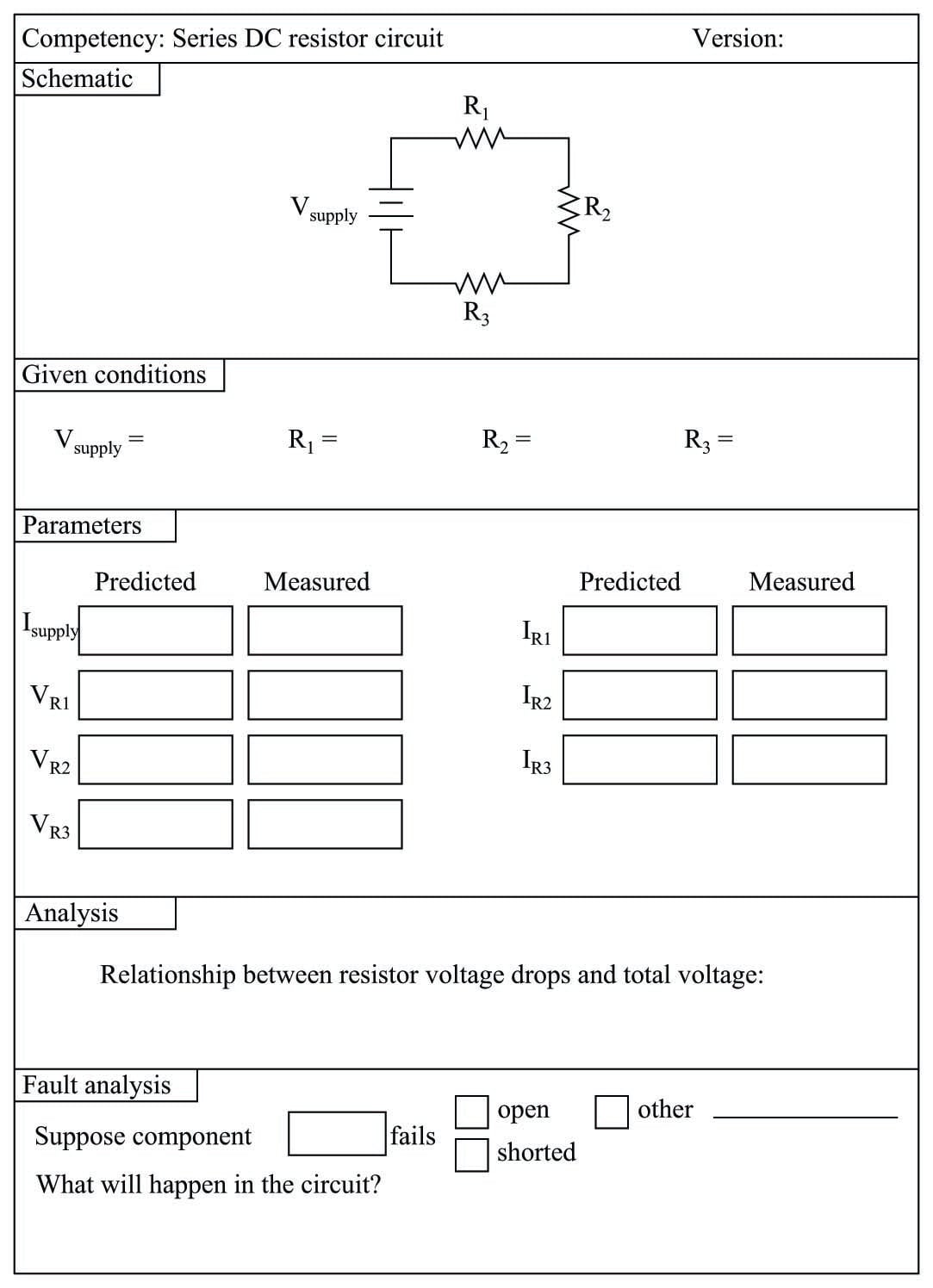
Note the Fault Analysis section at the end of this page. Here, after the instructor has verified the correctness of the student’s mathematical predictions and multimeter measurements, he or she would then challenge the student to predict the effects of a random component fault (either quantitatively or qualitatively), perhaps one of the resistors failing open or shorted. The student makes their predictions, then the instructor simulates that fault in the circuit (either by pulling the resistor out of the solderless breadboard to simulate an “open” or placing a jumper wire in parallel with the resistor to simulate a “short”). The student then uses his or her multimeter to verify the predictions. If the predicted results do not agree with the real measurements, the instructor works with the student to identify why their prediction(s) were faulty and hopefully correct any misconceptions leading to the incorrect result(s). Finally, a different component fault is chosen by the instructor, predictions made by the student, and verification made using a multimeter. The actual amount of time added to the instructor’s validation of student lab completion is relatively minor, but the benefits of exercising deductive diagnostic processes are great.
Example: predicting consequences of multiple faults
An example of a more advanced deductive diagnostic exercise appropriate to later phases of a student’s Instrumentation education appears here. A loop diagram shows a pressure recording system for an iso-butane distillation column:
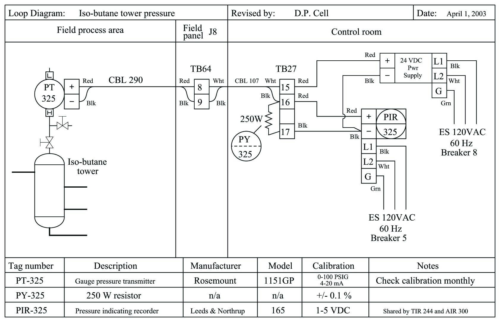
A set of questions accompanying this diagram challenge each student to predict effects in the instrument system resulting from known faults, such as:
- PT-325 block valve left shut and bleed valve left open (predict voltage between TB27-16 and TB27-17)
- Loose wire connection at TB64-9 (predict pressure indication at PIR-325)
- Circuit breaker #5 shut off (predict loop current at applied pressure of 50 PSI)
Given each hypothetical fault, there is only one correct conclusion for any given question. This makes deductive exercises unambiguous to assess.
Example: identifying possible faults
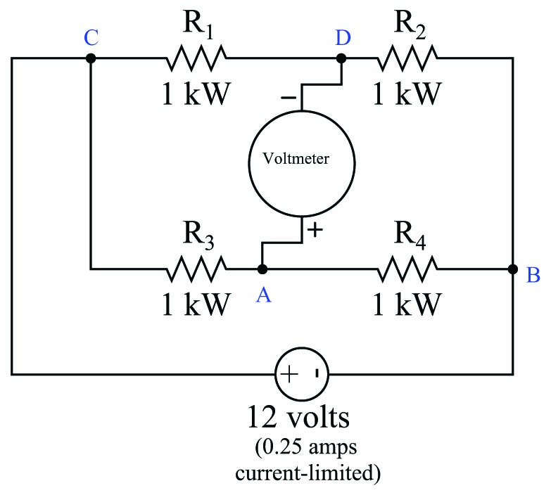
A more challenging type of deductive troubleshooting problem easily given in homework or on exams appears here. It asks students to examine a list of potential faults, marking each one of them as either “possible” or “impossible” based on whether or not each fault is independently capable of accounting for all symptoms in the system:
Suppose a voltmeter registers 6 volts between test points C and B in this series-parallel circuit:

| Fault | Possible | Impossible |
|---|---|---|
| $R_1$ failed open | ||
| $R_2$ failed open | ||
| $R_3$ failed open | ||
| $R_1$ failed shorted | ||
| $R_2$ failed shorted | ||
| $R_3$ failed shorted | ||
| Voltage source dead |
This is still a deductive thinking exercise because each of the faults is given to the student, and it is a matter of deduction to determine whether or not each one of these proposed faults is capable of accounting for the symptoms. Students need only apply the general rules of electric circuits to tell whether or not each of these faults would cause the reported circuit behavior.
True to form for any deductive problem, there can only be one correct answer for each proposed fault. This makes the exercise easy and unambiguous to grade, while honing vitally important diagnostic skills.
One of the benefits of this kind of fault analysis problem is that it requires students to consider all consequences of a proposed fault. In order for one of the faults to be considered “possible,” it must account for all symptoms, not just one symptom. An example of this sort of problem is seen here:
Suppose the voltmeter in this circuit registers a strong negative voltage. A test using a digital multimeter (DMM) shows the voltage between test points D and B to be 6 volts:
| Fault | Possible | Impossible |
|---|---|---|
| $R_1$ failed open | ||
| $R_2$ failed open | ||
| $R_3$ failed open | ||
| $R_4$ failed open | ||
| $R_1$ failed shorted | ||
| $R_2$ failed shorted | ||
| $R_3$ failed shorted | ||
| $R_4$ failed shorted | ||
| Voltage source dead |
Several different faults are capable of causing the meter to read strongly negative (\(R_1\) short, \(R_2\) open, \(R_3\) open, \(R_4\) short), but only two are capable of this while not affecting the normal voltage (6 volts) between test points D and B: \(R_3\) open or \(R_4\) short. This simple habit of checking to see that the proposed fault accounts for all apparent conditions and not just some of them is essential for effective troubleshooting.
This same question format may be easily applied to most any system, not just electrical circuits. Consider this example, determining possible versus impossible faults on an exhaust scrubber system:
After years of successful operation, the level control loop in this exhaust scrubbing system begins to exhibit problems. The liquid level inside the scrubbing tower mysteriously drops far below setpoint, as indicated by the level gauge (LG) on the side of the scrubber. The operators have tried to rectify this problem by increasing the setpoint adjustment on the level controller (LC), to no avail. The level transmitter (LT) is calibrated 3 PSI at 0% (low) level and 15 PSI at 100% (high) level:
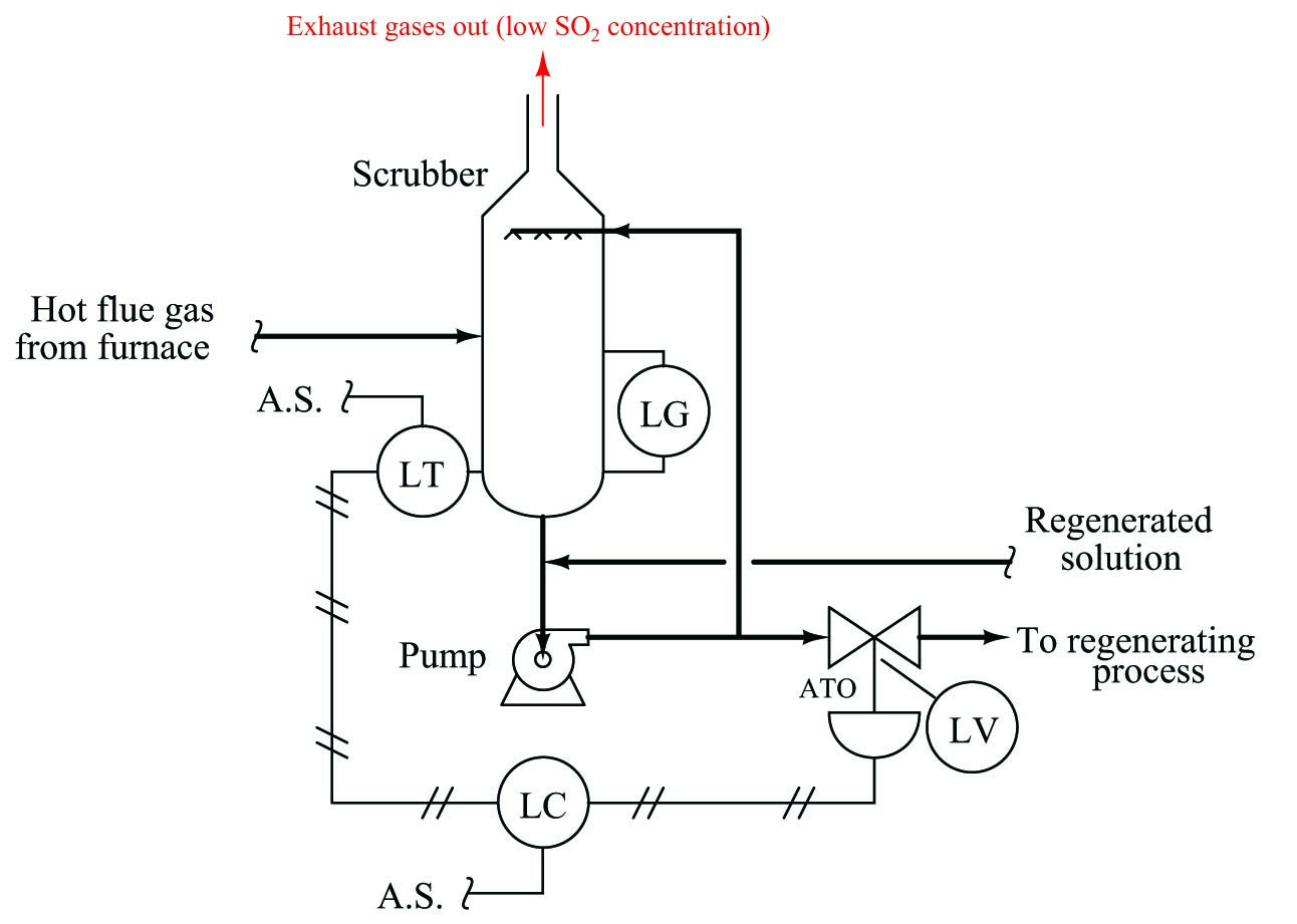
| Fault | Possible | Impossible |
|---|---|---|
| Air supply to LT shut off | ||
| Air supply to LC shut off | ||
| Pump shut off | ||
| Broken air line between LT and LC | ||
| Broken air line between LC and LV | ||
| Plugged nozzle inside LC | ||
| Plugged orifice inside LC | ||
| Leak in bottom of scrubber |
This exercise is particularly good because it requires the student to determine the action of the level controller (LC) before some of the proposed faults may be analyzed. In this case, the level controller must be direct-acting, so that an increasing liquid level inside the scrubber will cause an increasing air signal to the air-to-open (ATO) valve. letting more liquid out of the scrubber to stabilize the level. Without knowing that the level controller is direct-acting, it would be impossible to conclude the effect of a failed air supply to the level transmitter (LT), the first fault proposed in the table.
Example: assessing value of multiple diagnostic tests
A variation on this theme of determining the possibility of proposed faults is to assess the usefulness of proposed diagnostic tests. In other words, the student is presented with a scenario where something is amiss with a system, but instead of selecting a set of proposed faults as being either possible or impossible, the student must determine whether or not a set of proposed tests would be diagnostically relevant. An example of this in a simple series-parallel resistor circuit is shown here:
Suppose a voltmeter registers 0 volts between test points E and F in this circuit. Determine the diagnostic value of each of the following tests. Assume only one fault in the system, including any single component or any single wire/cable/tube connecting components together. If a proposed test could provide new information to help you identify the location and/or nature of the one fault, mark “yes.” Otherwise, if a proposed test would not reveal anything relevant to identifying the fault (already discernible from the measurements and symptoms given so far), mark “no.”

| Diagnostic test | Yes | No |
|---|---|---|
| Measure $V_{AC}$ with power applied | ||
| Measure $V_{JK}$ with power applied | ||
| Measure $V_{CK}$ with power applied | ||
| Measure $I_{R1}$ with power applied | ||
| Measure $I_{R2}$ with power applied | ||
| Measure $I_{R3}$ with power applied | ||
| Measure $R_{AC}$ with source disconnected from $R_1$ | ||
| Measure $R_{DF}$ with source disconnected from $R_1$ | ||
| Measure $R_{EG}$ with source disconnected from $R_1$ | ||
| Measure $R_{HK}$ with source disconnected from $R_1$ |
This form of diagnostic problem tends to be much more difficult to solve than simply determining the possibility of proposed faults. To solve this form of problem, the student must first determine all possible component faults, and then assess whether or not each proposed test would provide new information useful in identifying which of these possible faults is the actual fault.
In this example problem, there are really only a few possible faults: a dead source, an open resistor \(R_1\), a shorted resistor \(R_2\), a shorted resistor \(R_3\), or a broken wire (open connection) somewhere in the loop E-B-A-C-D-F.
The first proposed test – measuring voltage between points A and B – would be useful because it would provide different results given a dead source, open \(R_1\), shorted \(R_2\), or shorted \(R_3\) versus an open between A-E or between C-F. Any of the former faults would result in 0 volts between A and B, while any of the latter faults would result in full source voltage between A and B.
The next proposed test – measuring voltage between points J and K – would be useless because we already know what the result will be: 0 volts. This result of this proposed test will be the same no matter which of the possible faults causing 0 voltage between points E and F exists, which means it will shed no new light on the nature or location of the fault.
Despite being very challenging, this type of deductive diagnostic exercise is nevertheless easy to administer and unambiguous to grade, making it very suitable for written tests.
Inductive diagnostic exercises
Inductive reasoning is where a person derives general principles from a specific situation. In the context of instrumentation and control systems, this means having students propose faults to account for specific symptoms and data measured in systems. This is actual troubleshooting, as opposed to deductive diagnosis which is an enabling skill for effective troubleshooting.
While real hands-on exercises are best for developing inductive diagnostic skill, much learning and assessment may be performed in written form as well.
Example: proposing faults in loop diagram
This exam question is a sample of an inductive diagnosis exercise presented in written form:
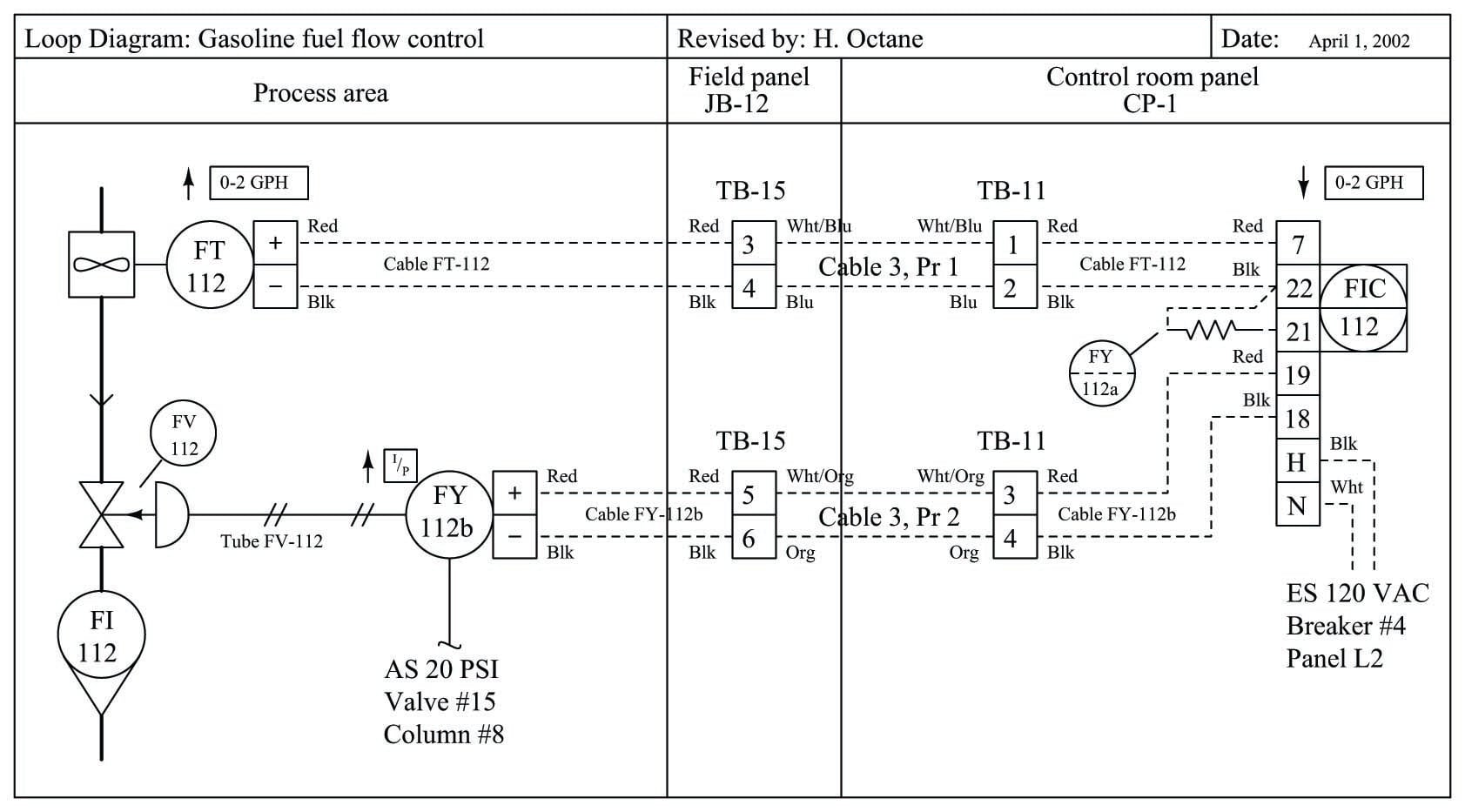
This system used to work just fine, but now it has a problem: the controller registers zero flow, and its output signal (to the valve) is saturated at 100% (wide open) as though it were trying to “ask” the valve for more flow. Your first diagnostic step is to check to see if there actually is gasoline flow through the flowmeter and valve by looking at the rotameter. The rotameter registers a flow rate in excess of 2 gallons per hour.
Identify possible faults in this system that could account for the controller’s condition (no flow registered, saturated 100% output), depending on what you find when you look at the rotameter:
- Possible fault:
- Possible fault:
Here, the student must identify two probably faults to account for all exhibited symptoms. More than two different kinds of faults are possible1122, but the student need only identify two faults independently capable of causing the controller to register zero flow when it should be registering more than 2 GPH.
Example: “virtual troubleshooting”
An excellent supplement to any hands-on troubleshooting activities is to have students perform “virtual troubleshooting” with you, the instructor. This type of activity cannot be practiced alone, but requires the participation of someone who knows the answer. It may be done with individual students or with a group.
A “virtual troubleshooting” exercise begins with a schematic diagram of the system such as this, containing clearly labeled test points (and/or terminal blocks) for specifying the locations of diagnostic tests:

Each student has their own copy of the diagram, as does the instructor. The instructor has furthermore identified a realistic fault within this system, and has full knowledge of that fault’s effects. In other words, the instructor is able to immediately tell a student how much voltage will be read between any two test points, what the effect of jumpering a pair of test points will be, what will happen when a pushbutton is pressed, etc.
The activity begins with a brief synopsis of the system’s malfunction, narrated by the instructor. Students then propose diagnostic tests to the instructor, with the instructor responding back to each student the results of their tests. As students gather data on the problem, they should be able to narrow their search to find the fault, choosing appropriate tests to identify the precise nature and location of the fault. The instructor may then assess each student’s diagnostic performance based on the number of tests and their sequence.
When performed in a classroom with a large group of students, this is actually a lot of fun!
Example: realistic faults in solderless breadboards
Solderless breadboards are universally used in the teaching of basic electronics, because they allow students to quickly and efficiently build different circuits using replaceable components. As wonderful as breadboards are for fast construction of electronic circuits, however, it is virtually impossible to create a realistic component fault without the fault being evident to the student simply by visual inspection. In order for a breadboard to provide a realistic diagnostic scenario, you must find a way to hide the circuit while still allowing access to certain test points in the circuit.
A simple way to accomplish this is to build a “troubleshooting harness” consisting of a multi-terminal block connected to a multi-conductor cable. Students are given instructions to connect various wires of this cable to critical points in the circuit, then cover up the breadboard with a five-sided box so that the circuit can no longer be seen. Test voltages are measured between terminals on the block, not by touching test leads to component leads on the breadboard (since the breadboard is now inaccessible).
The following illustration shows what this looks like when applied to a single-transistor amplifier circuit:

If students cannot visually detect a fault, they must rely on voltage measurements taken from terminals on the block. This is quite challenging, as not even the shapes of the components may be seen with the box in place. The only guide students have for relating terminal block test points to points in the circuit is the schematic diagram, which is good practice because it forces students to interpret and follow the schematic diagram.
Example: realistic faults in a multi-loop instrument system
Whole instrumentation systems may also serve to build and assess individual diagnostic competence. In my lab courses, students work in teams to build functioning measurement and control loops using the infrastructure of a multiple-loop system (see Appendix section [multiple-loop system] beginning on page for a detailed description). Teamwork helps expedite the task of constructing each loop, such that even an inexperienced team is able to assemble a working loop (transmitter connected to an indicator or controller, with wires pulled through conduits and neatly landed on terminal blocks) in just a few hours.
Each student creates their own loop diagram showing all instruments, wires, and connection points, following ISA standards. These loop diagrams are verified by doing a “walk-through” of the loop with all student team members present. The “walk-through” allows the instructor to inspect work quality and ensure any necessary corrections are made to the diagrams. After each team’s loop has been inspected and all student loop diagrams edited, the diagrams are placed in a document folder accessible to all students in the lab area.
Once the loop is wired, calibrated, inspected, and documented, it is ready to be faulted. When a student is ready to begin their diagnostic exercise, they gather their team members and approach the instructor. The instructor selects a loop diagram from the document folder not drawn by that student, ideally of a loop constructed by another team. The student and teammates leave the lab room, giving the instructor time to fault the loop. Possible faults include:
- Loosen wire connections
- Short wire connections (loose strands of copper strategically placed to short adjacent terminals together)
- Cut cables in hard-to-see locations
- Connect wires to the wrong terminals
- Connect wire pairs backward
- Mis-configure instrument calibration ranges
- Insert square root extraction where it is not appropriate
- Mis-configure controller action or display
- Insert unrealistically large damping constants in either the transmitter, indicator, or final element
- Plug pneumatic signal lines with foam earplugs
- Turn off hand valves
- Trip circuit breakers
After the fault has been inserted, the instructor calls the student team back into the lab area (ideally using a hand-held radio, simulating the work environment of a large industrial facility where technicians carry two-way radios) to describe the symptoms. This part of the exercise works best when the instructor acts the part of a bewildered operator, describing what the system is not doing correctly, without giving any practical advice on the location of the problem or how to fix it1123. An important detail for the instructor to include is the “history” of the fault: is this a new loop which has never worked correctly, or was it a working system that failed? Faults such as mis-connected wires are realistic of improper installation (new loop), while faults such as loose connections are perfectly appropriate for previously working systems. Whether the instructor freely offers this “history” or waits for the student to ask, it is important to include in the diagnostic scenario because it is an extremely useful piece of information to know while troubleshooting actual systems in industry. Virtually anything may be wrong (including multiple faults) in a brand-new installation, whereas previously working systems tend to fail in fewer ways.
After this introduction, the one student begins his or her diagnosis, with the other team members acting as scribes to document the student’s steps. The diagnosing student may ask a teammate for manual assistance (e.g. operating a controller while the student observes a control valve’s motion), but no one is allowed to help the one student diagnose the problem. The instructor observes the student’s procedure while the student explains the rationale motivating each action, with only a short time given (typically 5 minutes) to determine the general location of the fault causing the problem (e.g. located in the transmitter, control valve, wiring, controller/DCS, tubing, etc.). If after that time period the student is unable to correctly isolate the general location, the exercise is aborted and the instructor reviews the student’s actions (as documented by the teammates) to help the student understand where they went wrong in their diagnosis. Otherwise, the student is given more time1124 to pinpoint the nature of the fault.
Depending on the sequencing of your students’ coursework, some diagnostic exercises may include components unfamiliar to the student. For example, a relatively new student familiar only with the overall function of a control loop but intimately familiar with the workings of measurement devices may be asked to troubleshoot a loop where the fault is in the control valve positioner rather than in the transmitter. I still consider this to be a fair assessment of the student’s diagnostic ability, so long as the expectations are commensurate with the student’s knowledge. I would not expect a student to precisely locate the nature of a positioner fault if they had never studied the function or configuration of a valve positioner, but I would expect them to be able to broadly identify the location of the fault (e.g. “it’s somewhere in the valve”) so long as they knew how a control signal is supposed to command a control valve to move. That student should be able to determine by manually adjusting the controller output and measuring the output signal with the appropriate loop-testing tools that the valve was not responding as it should despite the controller properly performing its function. The ability to diagnose problems in instrument systems where some components of the system are mysterious “black boxes” is a very important skill, because your students will have to do exactly that when they step into industry and work with specific pieces of equipment they never had time to learn about in school1125.
I find it nearly impossible to fairly assign a letter or percentage grade to any particular troubleshooting effort, because no two scenarios are quite the same. Mastery assessment (either pass or fail, with multiple opportunities to re-try) seems a better fit. Mastery assessment with no-penalty retries also enjoys the distinct advantage of directing needed attention toward and providing more practice for weaker students: the more a student struggles with troubleshooting, the more they must exercise those skills.
Successfully passing a troubleshooting exercise requires not only that the fault be correctly identified and located in a timely manner, but that all steps leading to the diagnosis are logically justified. Random “trial and error” tests by the student will result in a failed attempt, even if the student was eventually able to locate the fault. A diagnosis with no active tests such as multimeter or test gauge measurements, or actions designed to stimulate system components, will also fail to pass. For example, a student who successfully locates a bad wiring connection by randomly tugging at every wire connection should not pass the troubleshooting exercise because such actions do not demonstrate diagnostic thinking1126.
To summarize key points of diagnostic exercises using a multiple-loop system:
- Students work in teams to build each loop
- Loop inspection and documentation finalized by a “walk-through” with the instructor
- Instructor placement of faults (it is important no student knows what is wrong with the loop!)
- Each student individually diagnoses a loop, with team members acting merely as scribes
- Students must use loop diagrams drawn by someone else, ideally diagnosing a loop built by a different team
- Brief time limit for each student to narrow the scope of the problem to a general location in the system
- Passing a diagnostic exercise requires: \(\rightarrow\) Accurate identification of the problem \(\rightarrow\) Each diagnostic step logically justified by previous results \(\rightarrow\) Tests (measurements, component response checks) performed before reaching conclusions
- Mastery (pass/fail) assessment of each attempt, with multiple opportunities for re-tries if necessary
