 Facebook
 Google
 GitHub
 Linkedin
Self-regulating, Integrating, and Runaway Process Characteristics
Perhaps the most important rule of controller tuning is to know the process before attempting to adjust the controller’s tuning. Unless you adequately understand the nature of the process you intend to control, you will have little hope in actually controlling it well. This section of the book is dedicated to an investigation of different process characteristics and how to identify each.
Quantitative PID tuning methods (see section 30.3 beginning on page ) attempt to map the characteristics of a process so good PID parameters may be chosen for the controller. The goal of this section is for you to understand various process types by observation and qualitative analysis so you may comprehend why different tuning parameters are necessary for each type, rather than mindlessly following a step-by-step PID tuning procedure.
The three major classifications of process response are self-regulating, integrating, and runaway. Each of these process types is defined by its response to a step-change in the manipulated variable (e.g. control valve position or state of some other final control element). A “self-regulating” process responds to a step-change in the final control element’s status by settling to a new, stable value. An “integrating” process responds by ramping either up or down at a rate proportional to the magnitude of the final control element’s step-change. Finally, a “runaway” process responds by ramping either up or down at a rate that increases over time, headed toward complete instability without some form of corrective action from the controller.
Self-regulating, integrating, and runaway processes have very different control needs. PID tuning parameters that may work well to control a self-regulating process, for example, will not work well to control an integrating or runaway process, no matter how similar any of the other characteristics of the processes may be951. By first identifying the characteristics of a process, we may draw some general conclusions about the P, I, and D setting values necessary to control it well.
Perhaps the best method for testing a process to determine its natural characteristics is to place the controller in manual mode and introduce a step-change to the controller output signal. It is critically important that the loop controller be in manual mode whenever process characteristics are being explored. If the controller is left in the automatic mode, the response seen from the process to a setpoint or load change will be partly due to the natural characteristics of the process itself and partly due to the corrective action of the controller. The controller’s corrective action thus interferes with our goal of exploring process characteristics. By placing the controller in “manual” mode, we turn off its corrective action, effectively removing its influence by breaking the feedback loop between process and controller, controller and process. In manual mode, the response we see from the process to an output (manipulated variable) or load change is purely a function of the natural process dynamics, which is precisely what we wish to discern.
A test of process characteristics with the loop controller in manual mode is often referred to as an open-loop test, because the feedback loop has been “opened” and is no longer a complete loop. Open-loop tests are the fundamental diagnostic technique applied in the following subsections.
Self-regulating processes
If a liquid flow-control valve is opened in a step-change fashion, flow through the pipe tends to self-stabilize at a new rate very quickly. The following illustration shows a typical liquid flow-control installation, with a process trend showing the flow response following a manual-mode (also known as “open-loop”) step-change in valve position:
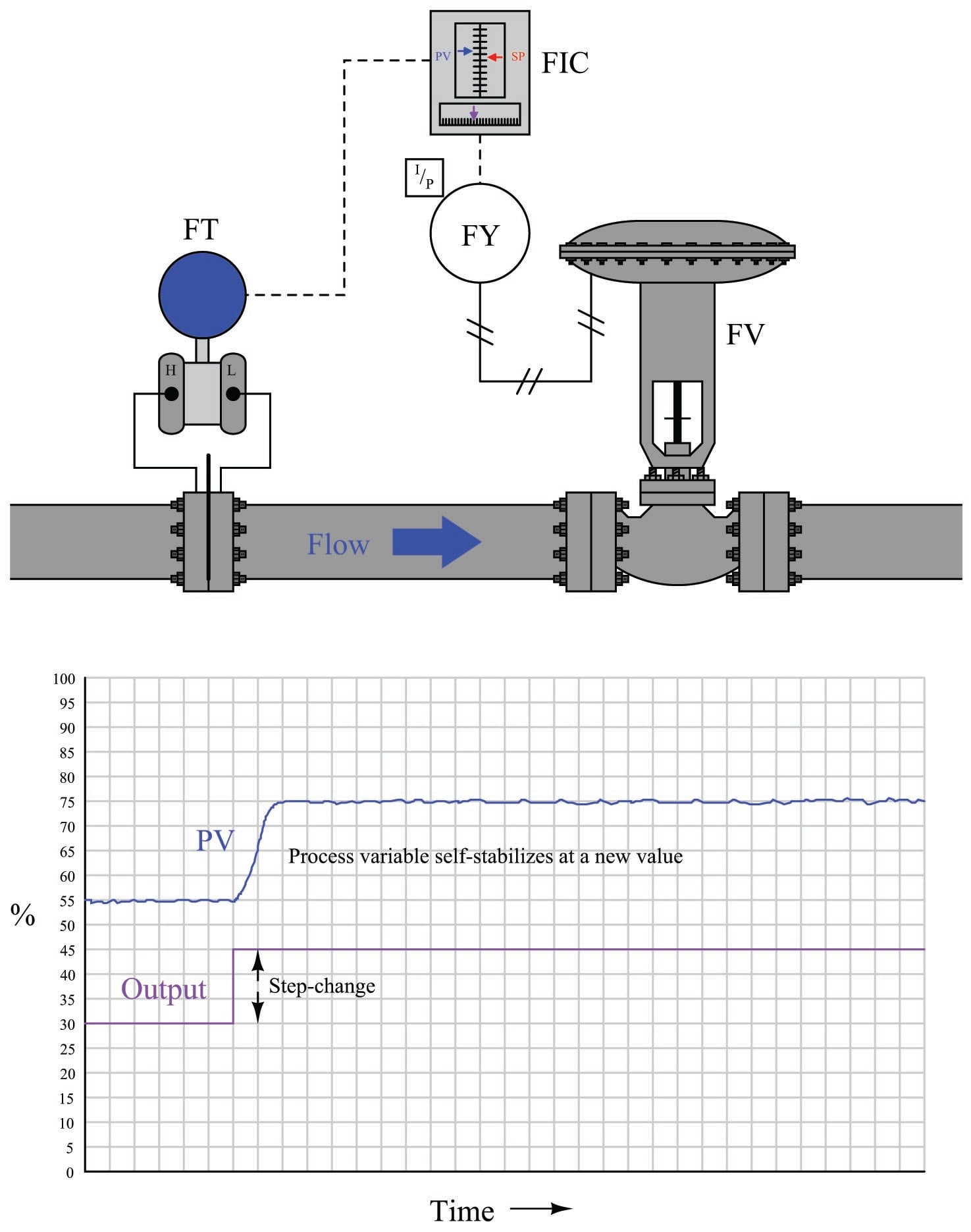
The defining characteristic of a self-regulating process is its inherent ability to settle at a new process variable value without any corrective action on the part of the controller. In other words, a self-regulating process will exhibit a unique process variable value for each possible output (valve) value. The inherently fast response of a liquid flow control process makes its self-regulating nature obvious: the self-stabilization of flow generally takes place within a matter of seconds following the valve’s motion. Many other processes besides liquid flow are self-regulating as well, but their slow response times require patience on the part of the observer to tell that the process will indeed self-stabilize following a step-change in valve position.
A corollary to the principle of self-regulation is that a unique output value will be required to achieve a new process variable value. For example, to achieve a greater flow rate, the control valve must be opened further and held at that further-open position for as long as the greater flow rate is desired. This presents a fundamental problem for a proportional-only controller. Recall the formula for a proportional-only controller, defining the output value (\(m\)) by the error (\(e\)) between process variable and setpoint multiplied by the gain (\(K_p\)) and added to the bias (\(b\)):
\[m = K_p e + b\]
Where,
\(m\) = Controller output
\(e\) = Error (difference between PV and SP)
\(K_p\) = Proportional gain
\(b\) = Bias
Suppose we find the controller in a situation where there is no error (PV = SP), and the flow rate is holding steady at some value. If we then increase the setpoint value (calling for a greater flow rate), the error will increase, driving the valve further open. As the control valve opens further, flow rate naturally increases to match. This increase in process variable drives the error back toward zero, which in turn causes the controller to decrease its output value back toward where it was before the setpoint change. However, the error can never go all the way back to zero because if it did, the valve would return to its former position, and that would cause the flow rate to self-regulate back to its original value before the setpoint change was made. What happens instead is that the control valve begins to close as flow rate increases, and eventually the process finds some equilibrium point where the flow rate is steady at some value less than the setpoint, creating just enough error to drive the valve open just enough to maintain that new flow rate. Unfortunately, due to the need for an error to exist, this new flow rate will fall shy of our setpoint. We call this error proportional-only offset, or droop, and it is an inevitable consequence of a proportional-only controller attempting to control a self-regulating process.
For any fixed bias value, there will be only one setpoint value that is perfectly achievable for a proportional-only controller in a self-regulating process. Any other setpoint value will result in some degree of offset in a self-regulating process. If dynamic stability is more important than absolute accuracy (zero offset) in a self-regulating process, a proportional-only controller may suffice. A great many self-regulating processes in industry have been and still are controlled by proportional-only controllers, despite some inevitable degree of offset between PV and SP.
The amount of offset experienced by a proportional-only controller in a self-regulating process may be minimized by increasing the controller’s gain. If it were possible to increase the gain of a proportional-only controller to infinity, it would be able to achieve any setpoint desired with zero offset! However, there is a practical limit to the extent we may increase the gain value, and that limit is oscillation. If a controller is configured with too much gain, the process variable will begin to oscillate over time, never stabilizing at any value at all, which of course is highly undesirable for any automatic control system. Even if the gain is not great enough to cause sustained oscillations, excessive values of gain will still cause problems by causing the process variable to oscillate with decreasing amplitude for a period of time following a sudden change in either setpoint or load. Determining the optimum gain value for a proportional-only controller in a self-regulating process is, therefore, a matter of compromise between excessive offset and excessive oscillation.
Recall that the purpose of integral (or “reset”) control action was the elimination of offset. Integral action works by ramping the output of the controller at a rate determined by the magnitude of the offset: the greater the difference between PV and SP for an integral controller, the faster that controller’s output will ramp over time. In fact, the output will stabilize at some value only if the error is diminished to zero (PV = SP). In this way, integral action works tirelessly to eliminate offset.
It stands to reason then that a self-regulating process absolutely requires some amount of integral action in the controller in order to achieve zero offset for all possible setpoint values. The more aggressive (faster) a controller’s integral action, the sooner offset will be eliminated. Just how much integral action a self-regulating process can tolerate depends on the magnitudes of any time lags in the system. The faster a process’s natural response is to a manual step-change in controller output, the better it will respond to aggressive integral controller action once the controller is placed in automatic mode. Aggressive integral control action in a slow process, however, will result in oscillation due to integral wind-up952.
It is not uncommon to find self-regulating processes being controlled by integral-only controllers. An “integral-only” process controller is an instrument lacking proportional or derivative control modes. Liquid flow control is a nearly ideal candidate process for integral-only control action, due to its self-regulating and fast-responding nature.
Summary:
- Self-regulating processes are characterized by their natural ability to stabilize at a new process variable value following changes in the control element value or load(s).
- Self-regulating processes absolutely require integral controller action to eliminate offset between process variable and setpoint, because only integral action is able to create a different controller output value once the error returns to zero.
- Faster integral controller action results in quicker elimination of offset.
- The amount of integral controller action tolerable in a self-regulating process depends on the degree of time lag in the system. Too much integral action will result in oscillation, just like too much proportional control action.
Integrating processes
A good example of an integrating process is liquid level control, where either the flow rate of liquid into or out of a vessel is constant and the other flow rate varies. If a control valve is opened in a step-change fashion, liquid level in the vessel ramps at a rate proportional to the difference in flow rates in and out of the vessel. The following illustration shows a typical liquid level-control installation, with a process trend showing the level response to a step-change in valve position (with the controller in manual mode, for an “open-loop” test):
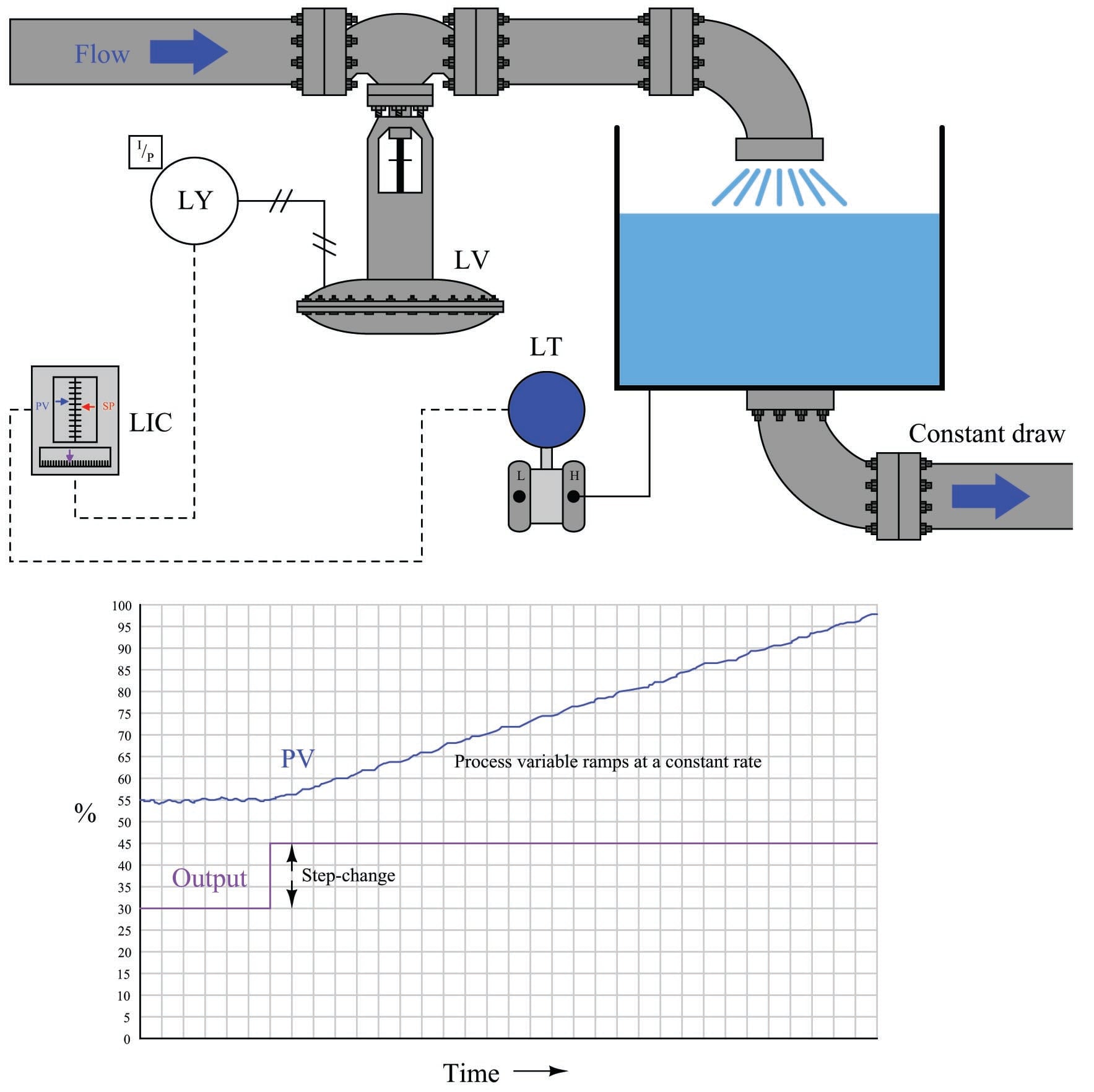
It is critically important to realize that this ramping action of the process variable over time is a characteristic of the process itself, not the controller. When liquid flow rates in and out of a vessel are mis-matched, the liquid level within that vessel will change at a rate proportional to the difference in flow rates. The trend shown here reveals a fundamental characteristic of the process, not the controller (this should be obvious once it is realized that the step-change in output is something that would only ever happen with the controller in manual mode).
Mathematically, we may express the integrating nature of this process using calculus notation. First, we may express the rate of change of volume in the tank over time (\(dV \over dt\)) in terms of the flow rates in and out of the vessel:
\[{dV \over dt} = Q_{in} - Q_{out}\]
For example, if the flow rate of liquid going into the vessel was 450 gallons per minute, and the constant flow rate drawn out of the vessel was 380 gallons per minute, the volume of liquid contained within the vessel would increase over time at a rate equal to 70 gallons per minute: the difference between the in-flow and the out-flow rates.
Another way to express this mathematical relationship between flow rates and liquid volume in the vessel is to use the calculus function of integration:
\[\Delta V = \int_0^T (Q_{in} - Q_{out}) \> dt\]
The amount of liquid volume accumulated in the vessel (\(\Delta V\)) between time 0 and time \(T\) is equal to the sum (\(\int\)) of the products (multiplication) of difference in flow rates in and out of the vessel (\(Q_{in} - Q_{out}\)) during infinitesimal increments of time (\(dt\)).
In the given scenario of a liquid level control system where the out-going flow is held constant, this means the level will be stable only at one in-coming flow rate (where \(Q_{in} = Q_{out}\)). At any other controlled flow rate, the level will either be increasing over time or decreasing over time.
This process characteristic perfectly matches the characteristic of a proportional-only controller, where there is one unique output value when the error is zero (PV = SP). We may illustrate this by performing a “thought experiment” on the liquid level-control process shown earlier having a constant draw out the bottom of the vessel. Imagine this process controlled by a proportional-only controller in automatic mode, with the bias value (\(b\)) of the controller set to the exact value needed by the control valve to make in-coming flow exactly equal to the constant out-going flow (draw). This means that when the process variable is precisely equal to setpoint (PV = SP), the in-flow will match the out-flow and therefore the liquid level will hold constant. If now an operator were to increase the setpoint value (with the controller in automatic mode), it will cause the valve to open further, adding liquid at a faster rate to the vessel. The naturally integrating nature of the process will result in an increasing liquid level. As level increases, the amount of error in the controller decreases, causing the valve to approach its original (bias) position. When the level reaches the new setpoint, proportional-only action will return the controller output to its original (bias) value, thus returning the in-flow control valve to its original position. This return to the bias position makes in-flow once again equal to out-flow, and so the level remains constant at the new setpoint with absolutely no offset (“droop”) even though the controller only exhibits proportional action. Proportional-only offset exists in a self-regulating process because a new valve position is needed to achieve any new setpoint value. Proportional-only offset does not occur on setpoint changes in an integrating process because only one valve position is needed to hold the process variable constant at any setpoint value.
The more aggressive the controller’s proportional action, the sooner the integrating process will reach new setpoints. Just how much proportional action (gain) an integrating process can tolerate depends on the magnitudes of any time lags in the system as well as the magnitude of noise in the process variable signal. Any process system with time lags will oscillate if the controller has sufficient gain. Noise is a problem because proportional action directly reproduces process variable noise on the output signal: too much gain, and just a little bit of PV noise translates into a control valve whose stem position constantly jumps around.
Purely integrating processes do not require integral control action to eliminate offset as is the case with self-regulating processes, following a setpoint change. The natural integrating action of the process eliminates offset that would otherwise arise from setpoint changes. More than that, the presence of any integral action in the controller will actually force the process variable to overshoot setpoint following a setpoint change in a purely integrating process! Imagine a controller with integral action responding to a step-change in setpoint for the liquid level control process shown earlier. As soon as an error develops, the integral action will begin “winding up” the output value, forcing the valve to open more than proportional action alone would demand. By the time the liquid level reaches the new setpoint, the valve will have reached a position greater than where it originally was before the setpoint change953, which means the liquid level will not stop rising when it reaches setpoint, but in fact will overshoot setpoint. Only after the liquid level has spent sufficient time above setpoint will the integral action of the controller “wind” back down to its previous level, allowing the liquid level to finally achieve the new setpoint.
This is not to say that integral control action is completely unnecessary in integrating processes – far from it. If the integrating process is subject to load changes, only integral action can return the PV back to the SP value (eliminate offset). Consider, in our level control example, if the out-going flow rate were to change. Now, a new valve position will be required to achieve stable (unchanging) level in the vessel. A proportional-only controller is able to generate a new valve position only if an error develops between PV and SP. Without at least some degree of integral action configured in the controller, that error will persist indefinitely. Or consider if the liquid supply pressure upstream of the control valve were to change, resulting in a different rate of incoming flow for the same valve stem position as before. Once again, the controller would have to generate a different output value to compensate for this process change and stabilize liquid level, and the only way a proportional-only controller could do that is to let the process variable drift a bit from setpoint (the definition of an error or offset).
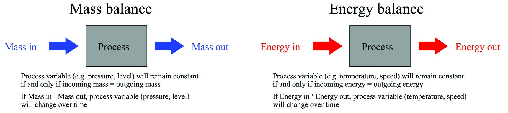
The example of an integrating process used here is just one of many possible processes where we are dealing with either a mass balance or an energy balance problem. “Mass balance” is the accounting of all mass into and out of a process. Since the Law of Mass Conservation states the impossibility of mass creation or destruction, all mass into and out of a process must be accounted for. If the mass flow rate into a process does not equal the mass flow rate out of a process, the process must be either gaining or losing an internal store of mass. The same may be said for energy: all energy flowing into and out of a process must be accounted for, since the Law of Energy Conservation states the impossibility of energy creation or destruction. If the energy flow rate (input power) into a process does not equal the energy flow rate (output power) out of a process, the process must be either gaining or losing an internal store of energy.
Common examples of integrating processes include the following:
- Liquid level control – mass balance – when the flow of liquid either into or out of a vessel is manipulated, and the other flows in or out of the vessel are constant
- Gas pressure control – mass balance – when the flow of gas either into or out of a vessel is manipulated, and the other flows in or out of the vessel are constant
- Storage bin level control – mass balance – when the conveyor feed rate into the bin is manipulated, and the draw from the bin is constant
- Temperature control – energy balance – when the flow of heat into or out of a process is manipulated, and all other heat flows are constant
- Speed control – energy balance – when the force (linear) or torque (angular) applied to a mass is manipulated, and all other loads are constant in force or torque
In a self-regulating process, the control element (valve) exerts control over both the in-flow and the out-flow of either mass or energy. In the previous subsection, where liquid flow control was the process example, the mass balance consisted of liquid flow into the valve and liquid flow out of the valve. Since the piping was essentially a “series” path for an incompressible fluid, where input flow must equal output flow at any given time, mass in and mass out were guaranteed to be in a state of balance, with one valve controlling both. This is why a change in valve position resulted in an almost immediate change and re-stabilization of flow rate: the valve exerts immediate control over both the incoming and the outgoing flow rates, with both in perfect balance. Therefore, nothing “integrates” over time in a liquid flow control process because there can never be an imbalance between in-flow and out-flow.
In an integrating process, the control element (valve) exerts control over either the in-flow or the out-flow of mass or energy, but never both. Thus, changing valve position in an integrating process causes an imbalance of mass flow and/or energy flow, resulting in the process variable ramping over time as either mass or energy accumulates in (or depletes from) the process.
Our “simple” example of an integrating (level-control) process becomes a bit more complicated if the outgoing flow depends on level, as is the case with a gravity-drained vessel where the outgoing flow is a function of liquid level in the vessel rather than being fixed at a constant rate as it was in the previous example:
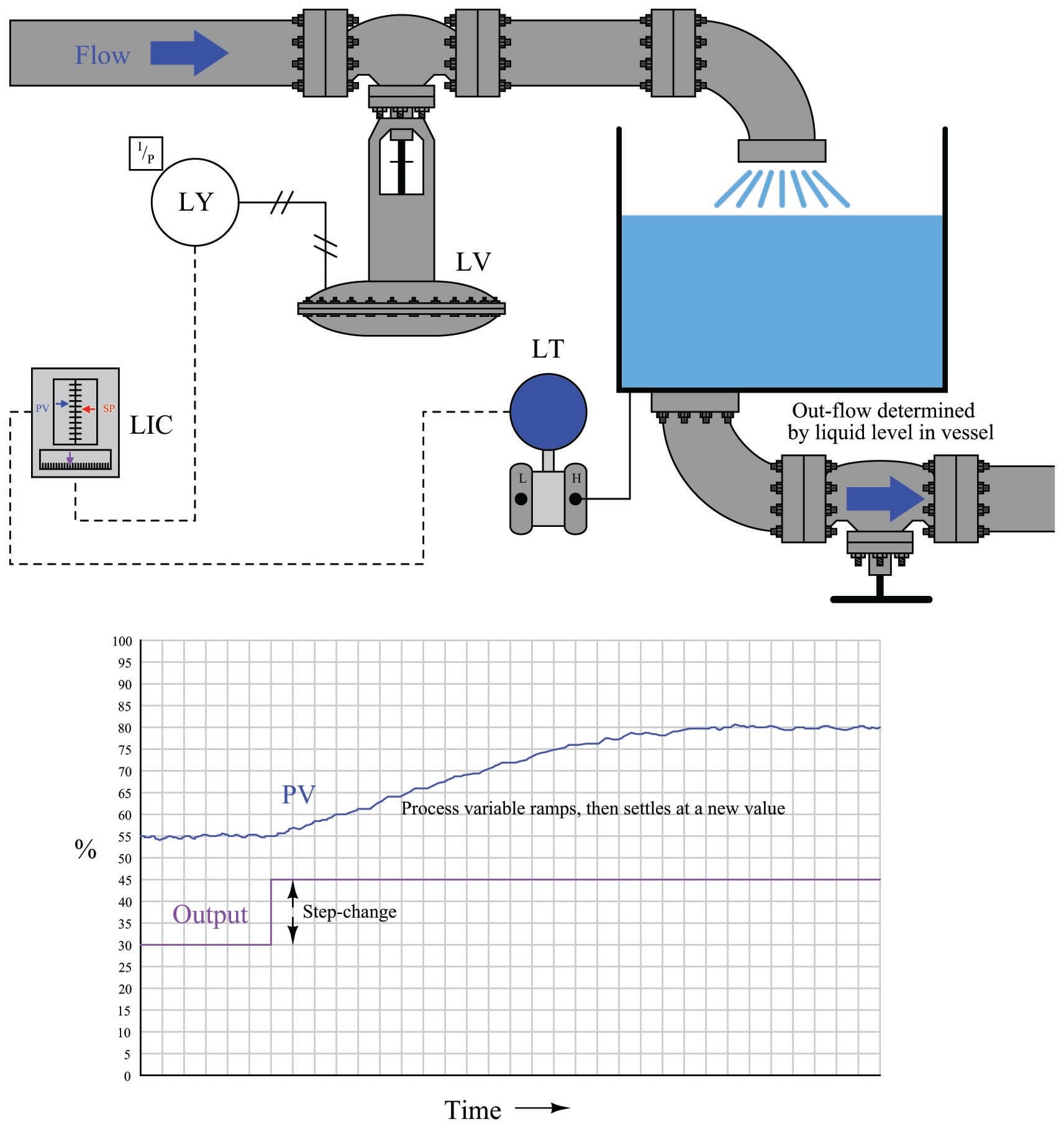
If we subject the control valve to a manual step-change increase, the flow rate of liquid into the vessel immediately increases. This causes an imbalance of incoming and outgoing flow, resulting in the liquid level rising over time. As level rises, however, increasing hydrostatic pressure across the manual valve at the vessel outlet causes the outgoing flow rate to increase. This causes the mass imbalance rate to be less than it was before, resulting in a decreased integration rate (rate of level rise). Thus, the liquid level still rises, but at a slower and slower rate as time goes on. Eventually, the liquid level will become high enough that the pressure across the manual valve forces a flow rate out of the vessel equal to the flow rate into the vessel. At this point, with matched flow rates, the liquid level stabilizes with no corrective action from the controller (remember, the step-change in output was made in manual mode!). Note the final result of letting the outgoing flow be a function of liquid level: what used to be an integrating process has now become a self-regulating process, albeit one with a substantial lag time.
Many processes ideally categorized as integrating actually behave in this manner. Although the manipulated variable may control the flow rate into or out of a process, the other flow rates often change with the process variable. Returning to our list of integrating process examples, we see how a PV-variable load in each case can make the process self-regulate:
- Liquid level control – mass balance – if the in-flow naturally decreases as liquid level rises and/or the out-flow naturally increases as liquid level rises, the vessel’s liquid level will tend to self-regulate instead of integrate
- Gas pressure control – mass balance – if in-flow naturally decreases as pressure rises and/or the out-flow naturally increases as pressure rises, the vessel’s pressure will tend to self-regulate instead of integrate
- Storage bin level control – mass balance – if the draw from the bin increases with bin level (greater weight pushing material out at a faster rate), the bin’s level will tend to self-regulate instead of integrate
- Temperature control – energy balance – if the process naturally loses heat at a faster rate as temperature increases and/or the process naturally takes in less heat as temperature rises, the temperature will tend to self-regulate instead of integrate
- Speed control – energy balance – if drag forces on the object increase with speed (as they usually do for any fast-moving object), the speed will tend to self-regulate instead of integrate
We may generalize all these examples of integrating processes turned self-regulating by noting the one aspect common to all of them: some natural form of negative feedback exists internally to bring the system back into equilibrium. In the mass-balance examples, the physics of the process ensure a new balance point will eventually be reached because the in-flow(s) and/or out-flow(s) naturally change in ways that oppose any change in the process variable. In the energy-balance examples, the laws of physics again conspire to ensure a new equilibrium because the energy gains and/or losses naturally change in ways that oppose any change in the process variable. The presence of a control system is, of course, the ultimate example of negative feedback working to stabilize the process variable. However, the control system may not be the only form of negative feedback at work in a process. All self-regulating processes are that way because they intrinsically possess some degree of negative feedback acting as a sort of natural, proportional-only control system.
This one detail completely alters the fundamental characteristic of a process from integrating to self-regulating, and therefore changes the necessary controller parameters. Self-regulation guarantees at least some integral controller action is necessary to attain new setpoint values. A purely integrating process, by contrast, requires no integral controller action at all to achieve new setpoints, and in fact is guaranteed to suffer overshoot following setpoint changes if the controller is programmed with any integral action at all! Both types of processes, however, need some amount of integral action in the controller in order to recover from load changes.
Summary:
- Integrating processes are characterized by a ramping of the process variable in response to a step-change in the control element value or load(s).
- This integration occurs as a result of either mass flow imbalance or energy flow imbalance in and out of the process.
- Integrating processes are ideally controllable with proportional controller action alone.
- Integral controller action guarantees setpoint overshoot in a purely integrating process.
- Some integral controller action will be required in integrating processes to compensate for load changes.
- The amount of proportional controller action tolerable in an integrating process depends on the degree of time lag and process noise in the system. Too much proportional action will result in oscillation (time lags) and/or erratic control element motion (noise).
- An integrating process will become self-regulating if sufficient negative feedback is naturally introduced. This usually takes the form of loads varying with the process variable.
Runaway processes
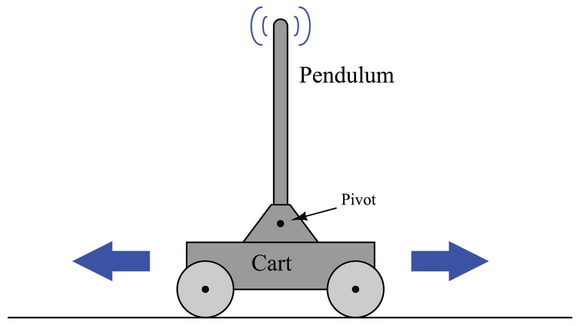
A classic “textbook” example of a runaway process is an inverted pendulum: a vertical stick balanced on its end by moving the bottom side-to-side. Inverted pendula are typically constructed in a laboratory environment by fixing a stick to a cart by a pivot, then equipping the cart with wheels and a reversible motor to give it lateral control ability. A sensor (usually a potentiometer) detects the stick’s angle from vertical, reporting that angle to the controller as the process variable. The cart’s motor is the final control element:
The defining characteristic of a runaway process is its tendency to accelerate away from a condition of stability with no corrective action applied. Viewed on a process trend, a runaway process tends to respond as follows to an open-loop step-change:
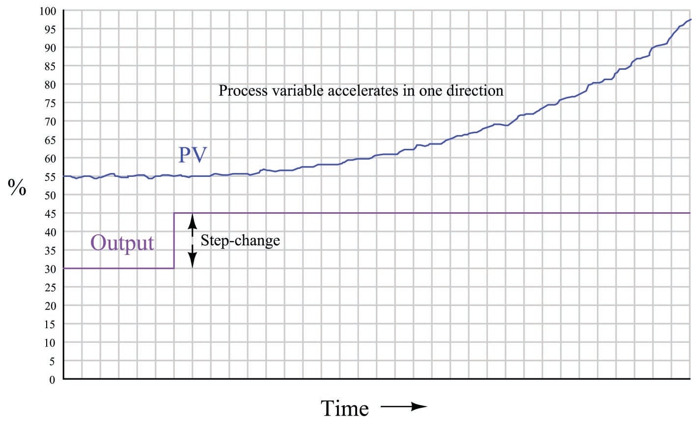
A synonym for “runaway” is negative self-regulation or negative lag, because the process variable curve over time for a runaway process resembles the mathematical inverse of a self-regulating curve with a lag time: it races away from the horizontal, while a self-regulating process variable draws closer and closer to the horizontal over time.
The “Segway\(^{TM}\)” personal transport device is a practical example of an inverted pendulum, with wheel motion controlled by a computer attempting to maintain the body of the vehicle in a vertical position. As the human rider leans forward, it causes the controller to spin the wheels with just the right amount of acceleration to maintain balance. There are many examples of runaway processes in motion-control applications, especially automated controls for vertical-flight vehicles such as helicopters and vectored-thrust aircraft such as the Harrier military fighter jet.
Some chemical reaction processes are runaway as well, especially exothermic (heat-releasing) reactions. Most chemical reactions increase in rate as temperature rises, and so exothermic reactions tend to accelerate with time (either becoming hotter or becoming colder) unless checked by some external influence. This poses a significant challenge to process control, as many exothermic reactions used to manufacture products must be temperature-controlled to ensure efficient production of the desired product. Off-temperature chemical reactions may not “favor” production of the desired products, producing unwanted byproducts and/or failing to efficiently consume the reactants. Furthermore, safety concerns usually surround exothermic chemical reactions, as no one wants their process to melt down or explode.
What makes a runaway process behave as it does is internal positive feedback. In the case of the inverted pendulum, gravity works to pull an off-center pendulum even farther off center, accelerating it until it falls down completely. In the case of exothermic chemical reactions, the direct relationship between temperature and reaction rate forms a positive feedback loop: the hotter the reaction, the faster it proceeds, releasing even more heat, making it even hotter. It should be noted that endothermic chemical reactions (absorbing heat rather than releasing heat) tend to be self-regulating for the exact same reason exothermic reactions tend to be runaway: reaction rate usually has a positive correlation with reaction temperature.
It is easy to demonstrate for yourself how challenging a runaway process can be to control. Simply try to balance a long stick vertically in the palm of your hand. You will find that the only way to maintain stability is to react swiftly to any changes in the stick’s angle – essentially applying a healthy dose of derivative control action to counteract any motion from vertical.
Fortunately, runaway processes are less common in the process industries. I say “fortunately” because these processes are notoriously difficult to control and usually pose more danger than inherently self-regulating processes. Many runaway processes are also nonlinear, making their behavior less intuitive to human operators.
Just as integrating processes may be forced to self-regulate by the addition of (natural) negative feedback, intrinsically runaway processes may also be forced to self-regulate given the presence of sufficient natural negative feedback. An interesting example of this is a pressurized water nuclear fission reactor.
Nuclear fission is a process by which the nuclei of specific types of atoms (most notably uranium-235 and plutonium-239) undergo spontaneous disintegration upon the absorption of an extra neutron, with the release of significant thermal energy and additional neutrons. A quantity of fissile material such as \(^{235}\)U or \(^{239}\)Pu is subjected to a source of neutron particle radiation, which initiates the fission process, releasing massive quantities of heat which may then be used to boil water into steam and drive steam turbine engines to generate electricity. The “chain reaction” of neutrons splitting fissile atoms, which then eject more neutrons to split more fissile atoms, is inherently exponential in nature. The more atoms split, the more neutrons are released, which then proceed to split even more atoms. The rate at which neutron activity within a fission reactor grows or decays over time is determined by the multiplication factor954, and this factor is easily controlled by the insertion of neutron-absorbing control rods into the reactor core.
Thus, a fission chain-reaction naturally behaves as an inverted pendulum. If the multiplication factor is greater than 1, the reaction grows exponentially. If the multiplication factor is less than 1, the reaction dies exponentially. In the case of a nuclear weapon, the desired multiplication factor is as large as physically possible to ensure explosive reaction growth. In the case of an operating nuclear power plant, the desired multiplication factor is exactly 1 to ensure stable power generation.
A simplified diagram of a pressurized-water reactor (PWR) is shown here:
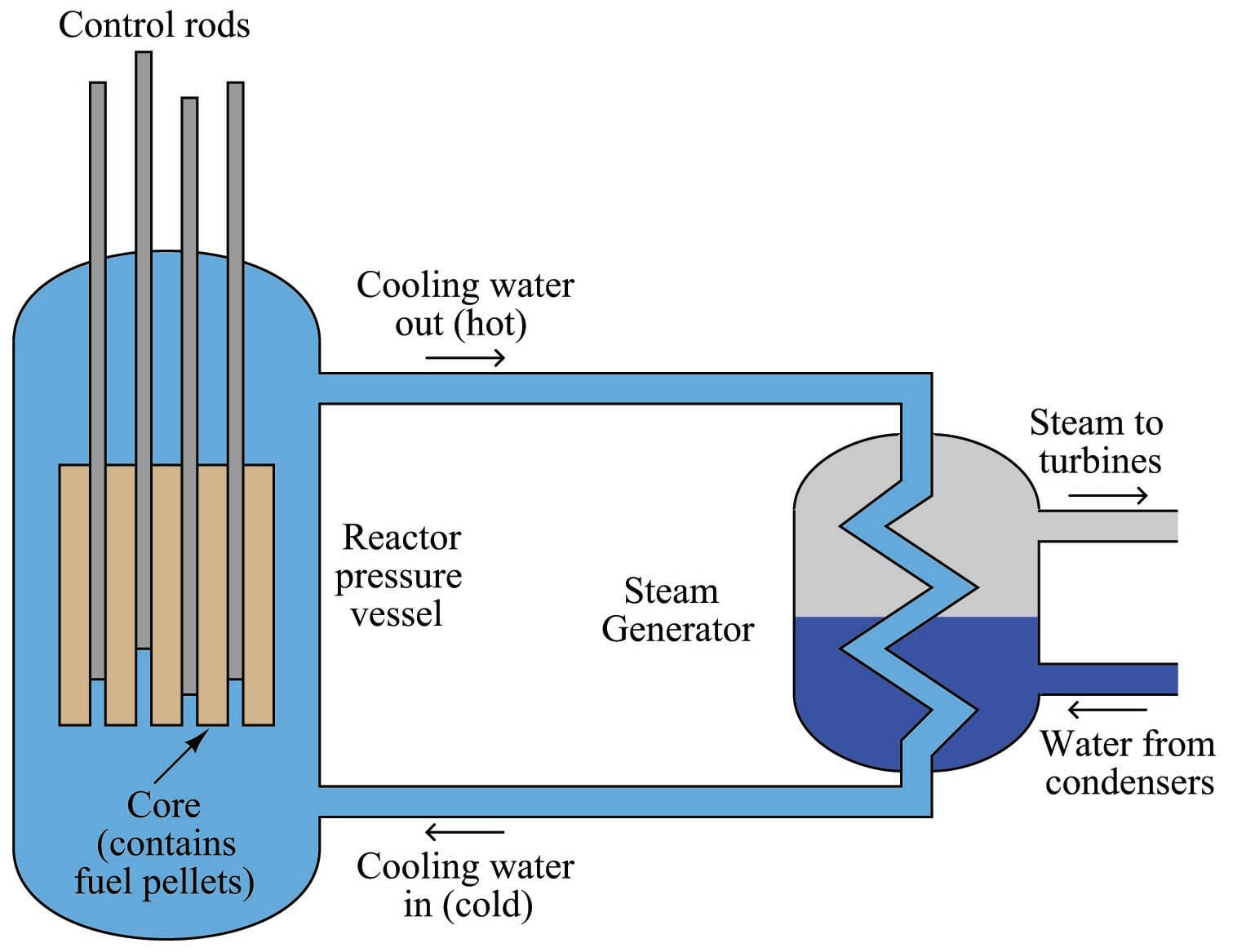
Water under high pressure (too high of pressure to boil) circulates through the reactor vessel, carrying heat away from the nuclear core, then transferring the heat energy to a heat exchanger (“steam generator”) where a second water loop is allowed to boil into steam and drive turbine engines to spin electrical generators. Control rods inserted into the core by linear actuators adjust the multiplication factor of the reactor.
If the multiplication factor of a fission reactor were solely controlled by the positions of these control rods, it would be a classic “runaway” process, with the reactor’s power level tending to increase toward infinity or decrease toward zero if the rods were at any position other than one yielding a multiplication factor of precisely unity (1). This would make nuclear reactors extremely difficult (if not impossible) to safely control. Fortunately, there are ways to engineer negative feedback directly into the design of the reactor core so that neutron activity naturally self-stabilizes without active control rod action. In water-cooled reactors, the water itself achieves this goal. Pressurized water plays a dual role in a fission reactor: it not only transfers heat out of the reactor core and into a boiler to produce steam, but it also offsets the multiplication factor inversely proportional to temperature. As the reactor core heats up, the water’s density changes, affecting the probability955 of neutrons being captured by fissile nuclei. This is called a negative temperature coefficient for the reactor, and it forces the otherwise runaway process of nuclear fission to become self-regulating.
With this self-regulating characteristic in effect, control rod position essentially determines the reactor’s steady-state temperature. The further the control rods are withdrawn from the core, the hotter the core will run. The cooling water’s natural negative temperature coefficient prevents the fission reaction from “running away” either to destruction or to shutdown.
Some nuclear fission reactor designs are capable of “runaway” behavior, though. The ill-fated reactor at Chernobyl (Ukraine, Russia) was of a design where its power output could “run away” under certain operating conditions, and that is exactly what happened on April 26, 1986. The Chernobyl reactor used solid graphite blocks as the main neutron-moderating substance, and as such its cooling water did not provide enough natural negative feedback to overcome the intrinsically runaway characteristic of nuclear fission. This was especially true at low power levels where the reactor was being tested on the day of the accident. A combination of poor management decisions, unusual operating conditions, and unstable design characteristics led to the reactor’s destruction with massive amounts of radiation released into the surrounding environment. It stands at the time of this writing as the world’s worst nuclear accident956.
Summary:
- Runaway processes are characterized by an exponential ramping of the process variable in response to a step-change in the control element value or load(s).
- This “runaway” occurs as a result of some form of positive feedback happening inside the process.
- Runaway processes cannot be controlled with proportional or integral controller action alone, and always requires derivative action for stability.
- Some integral controller action will be required in runaway processes to compensate for load changes.
- A runaway process will become self-regulating if sufficient negative feedback is naturally introduced, as is the case with water-moderated fission reactors.
Steady-state process gain
When we speak of a controller’s gain, we refer to the aggressiveness of its proportional control action: the ratio of output change to input change. However, we may go a step further and characterize each component within the feedback loop as having its own gain (a ratio of output change to input change):

The gains intrinsic to the measuring device (transmitter), final control device (e.g. control valve), and the process itself are all important in helping to determine the necessary controller gain to achieve robust control. The greater the combined gain of transmitter, process, and valve, the less gain is needed from the controller. The less combined gain of transmitter, process, and valve, the more gain will be needed from the controller. This should make some intuitive sense: the more “responsive” a process appears to be, the less aggressive the controller needs to be in order to achieve stable control (and vice-versa).
These combined gains may be empirically determined by means of a simple test performed with the controller in manual mode, also known as an “open-loop” test. By placing the controller in manual mode (and thus disabling its automatic correction of process changes) and adjusting the output signal by some fixed amount, the resulting change in process variable may be measured and compared. If the process is self-regulating, a definite ratio of PV change to controller output change may be determined.
For instance, examine this process trend graph showing a manual “step-change” and process variable response:
Here, the output step-change is 10% of scale, while the resulting process variable step-change is about 7.5%. Thus, the “gain” of the process957 (together with transmitter and final control element) is approximately 0.75, or 75% (Gain = \({7.5\% \over 10\%}\)). Incidentally, it is irrelevant that the PV steps down in response to the controller output stepping up. All this means is the process is reverse-responding, which necessitates direct action on the part of the controller in order to achieve negative feedback. When we calculate gains, we usually ignore directions (mathematical signs) and speak in terms of absolute values.
We commonly refer to this gain as the steady-state gain of the process, because the determination of gain is made after the PV settles to its self-regulating value.
Since from the controller’s perspective the individual gains of transmitter, final control element, and physical process meld into one over-all gain value, the process may be made to appear more or less responsive (more or less steady-state gain) just by altering the gain of the transmitter and/or the gain of the final control element.
Consider, for example, if we were to reduce the span of the transmitter in this process. Suppose this was a flow control process, with the flow transmitter having a calibrated range of 0 to 200 liters per minute (LPM). If a technician were to re-range the transmitter to a new range of 0 to 150 LPM, what effect would this have on the apparent process gain?
To definitively answer this question, we must re-visit the process trend graph for the old calibrated range:
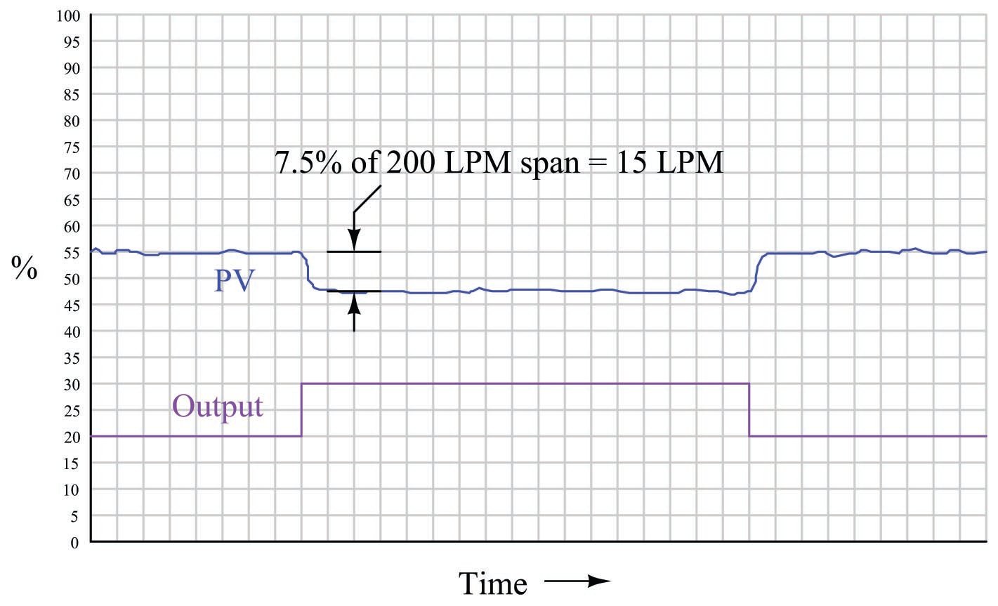
We see here that the 7.5% PV step-change equates to a change of 15 LPM given the flow transmitter’s span of 200 LPM. However, if a technician re-ranges the flow transmitter to have just three-quarters that amount of span (150 LPM), the exact same amount of output step-change will appear to have a more dramatic effect on flow, even though the physical response of the process has the same as it was before:
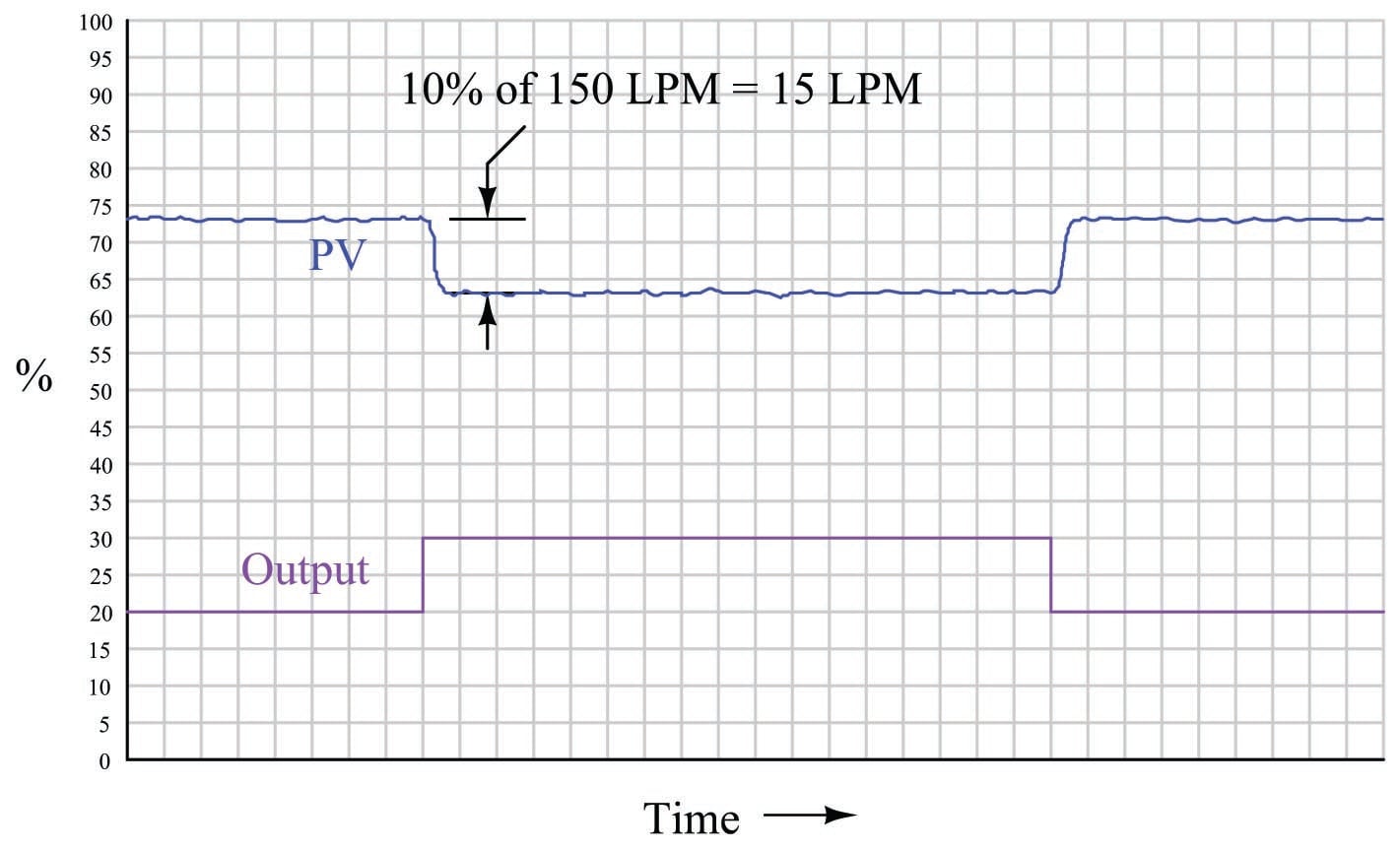
From the controller’s perspective – which only “knows” percent958 of signal range – the process gain appears to have increased from 0.75 to 1, with nothing more than a re-ranging of the transmitter. Since the process is now “more responsive” to controller output signals than it was before, there may be a tendency for the loop to oscillate in automatic mode even if it did not oscillate previously with the old transmitter range. A simple fix for this problem is to decrease the controller’s gain by the same factor that the process gain increased: we need to make the controller’s gain \(3 \over 4\) what it was before, since the process gain is now \(4 \over 3\) what it was before.
The exact same effect occurs if the final control element is re-sized or re-ranged. A control valve that is replaced with one having a different \(C_v\) value, or a variable-frequency motor drive that is given a different speed range for the same 4-20 mA control signal, are two examples of final control element changes which will result in different overall gains. In either case, a given change in controller output signal percentage results in a different amount of influence on the process thanks to the final control element being more or less influential than it was before. Re-tuning of the controller may be necessary in these cases to preserve robust control.
If and when re-tuning is needed to compensate for a change in loop instrumentation, all control modes should be proportionately adjusted. This is automatically done if the controller uses the Ideal or ISA PID equation, or if the controller uses the Series or Interacting PID equation959. All that needs to be done to an Ideal-equation controller in order to compensate for a change in process gain is to change that controller’s proportional (P) constant setting. Since this constant directly affects all terms of the equation, the other control modes (I and D) will be adjusted along with the proportional term. If the controller happens to be executing the Parallel PID equation, you will have to manually alter all three constants (P, I, and D) in order to compensate for a change in process gain.
A very important aspect of process gain is how consistent it is over the entire measurement range. It is entirely possible (and in fact very likely) that a process may be more responsive (have higher gain) in some areas of control than in others. Take for instance this hypothetical trend showing process response to a series of manual-mode step-changes:
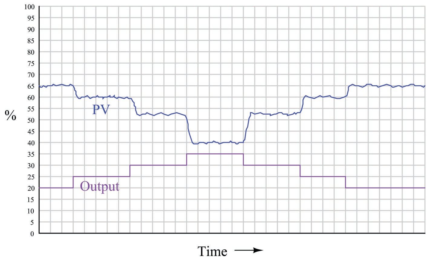
Note how the PV changes about 5% for the first 5% step-change in output, corresponding to a process gain of 1. Then, the PV changes about 7.5% for the next 5% output step-change, for a process gain of 1.5. The final increasing 5% step-change yields a PV change of about 12.5%, a process gain of 2.5. Clearly, the process being controlled here is not equally responsive throughout the measurement range. This is a concern to us in tuning the PID controller because any set of tuning constants that work well to control the process around a certain setpoint may not work as well if the setpoint is changed to a different value, simply because the process may be more or less responsive at that different process variable value.
Inconsistent process gain is a problem inherent to many different process types, which means it is something you will need to be aware of when investigating a process prior to tuning the controller. The best way to reveal inconsistent process gain is to perform a series of step-changes to the controller output while in manual mode, “exploring” the process response throughout the safe range of operation.
Compensating for inconsistent process gain is much more difficult than merely detecting its presence. If the gain of the process continuously grows from one end of the range to the other (e.g. low gain at low output values and high gain at high output values, or vice-versa), a control valve with a different characteristic may be applied to counter-act the process gain.
If the process gain follows some pattern more closely related to PV value rather than controller output value, the best solution is a type of controller known as an adaptive gain controller. In an adaptive gain controller, the proportional setting is made to vary in a particular way as the process changes, rather than be a fixed constant set by a human technician or engineer.
Lag time
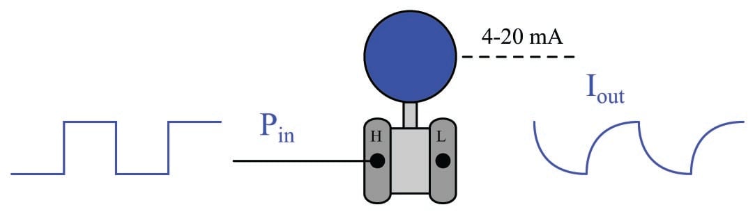
If a square-wave signal is applied to an RC passive integrator circuit, the output signal will appear to have a “sawtooth” shape, the crisp rising and falling edges of the square wave replaced by damped curves:
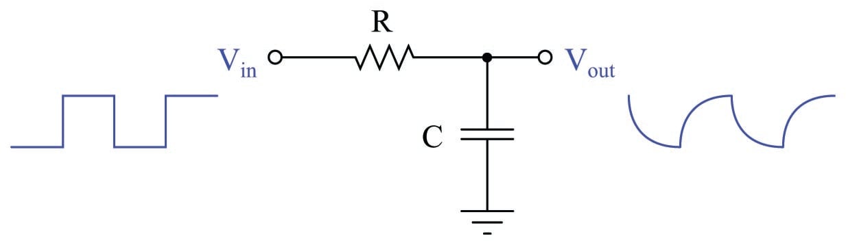
In a word, the output signal of this circuit lags behind the input signal, unable to keep pace with the steep rising and falling edges of the square wave.
Most mechanical and chemical processes exhibit a similar tendency: an “inertial” opposition to rapid changes. Even instruments themselves naturally960 damp sudden stimuli. We could have just as easily subjected a pressure transmitter to a series of pressure pulses resembling square waves, and witnessed the output signal exhibit the same damped response:
The gravity-drained level-control process highlighted in an earlier subsection exhibits a very similar response to a sudden change in control valve position:
For any particular flow rate into the vessel, there will be a final (self-regulating) point where the liquid level “wants” to settle961. However, the liquid level does not immediately achieve that new level if the control valve jumps to some new position, owing to the “capacity” of the vessel and the dynamics of gravity flow.
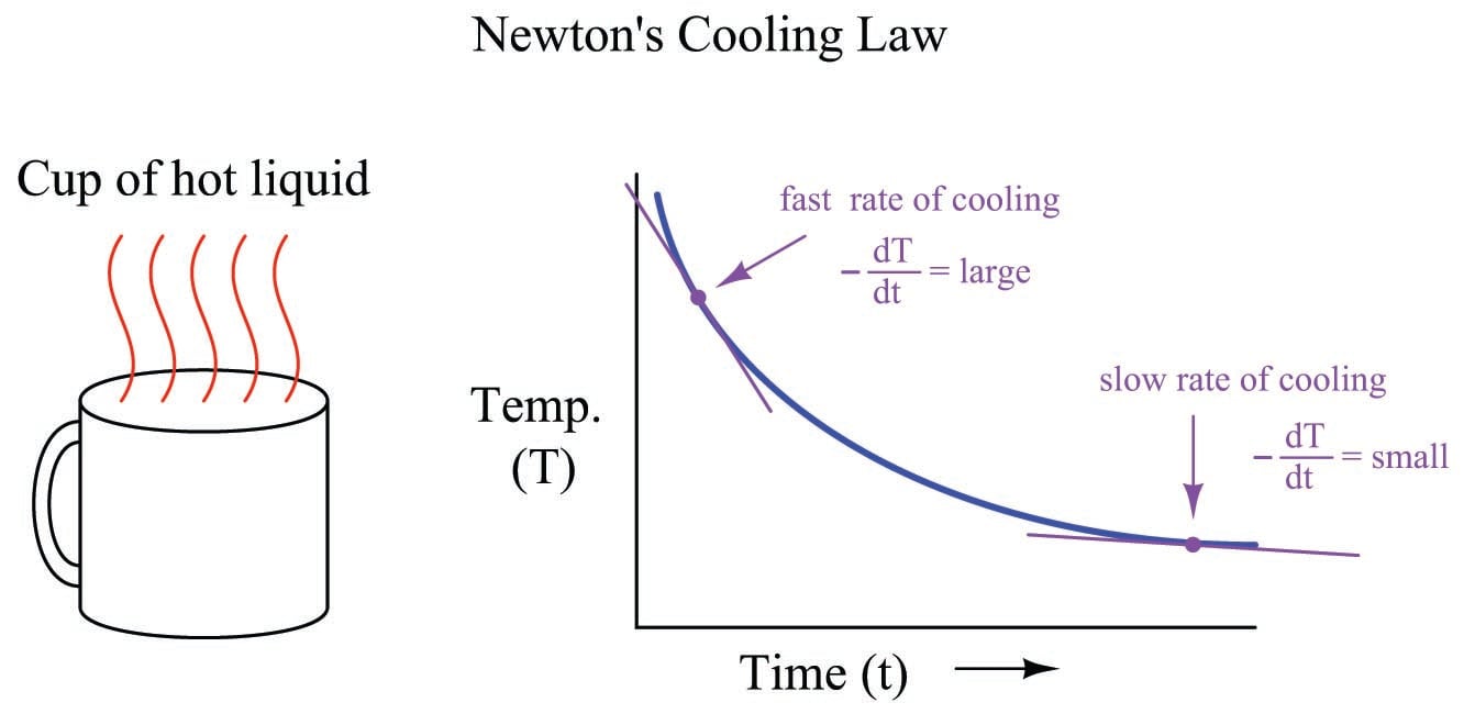
Any physical behavior exhibiting the same “settling” behavior over time may be said to illustrate a first-order lag. A classic “textbook” example of a first-order lag is the temperature of a cup of hot liquid, gradually equalizing with room temperature. The liquid’s temperature drops rapidly at first, but then slows its approach to ambient temperature as time progresses. This natural tendency is described by Newton’s Law of Cooling, mathematically represented in the form of a differential equation (an equation containing a variable along with one or more of its derivatives). In this case, the equation is a first-order differential equation, because it contains the variable for temperature (\(T\)) and the first derivative of temperature (\(dT \over dt\)) with respect to time:
\[{dT \over dt} = -k (T - T_{ambient})\]
Where,
\(T\) = Temperature of liquid in cup
\(T_{ambient}\) = Temperature of the surrounding environment
\(k\) = Constant representing the thermal conductivity of the cup
\(t\) = Time
All this equation tells us is that the rate of cooling (\(dT \over dt\)) is directly proportional (\(-k\)) to the difference in temperature between the liquid and the surrounding air (\(T - T_{ambient}\)). The hotter the temperature, the faster the object cools (the faster rate of temperature fall):
The proportionality constant in this equation (\(k\)) represents how readily thermal energy escapes the hot cup. A cup with more thermal insulation, for example, would exhibit a smaller \(k\) value (i.e. the rate of temperature loss \(dT \over dt\) will be less for any given temperature difference between the cup and ambient \(T - T_{ambient}\)).
A general solution to this equation is as follows:
\[T = \left( T_{initial} - T_{final} \right) \left( e^{-{t \over \tau}} \right) + T_{final}\]
Where,
\(T\) = Temperature of liquid in cup at time \(t\)
\(T_{initial}\) = Starting temperature of liquid (\(t = 0\))
\(T_{final}\) = Ultimate temperature of liquid (ambient)
\(e\) = Euler’s constant
\(\tau\) = “Time constant” of the system
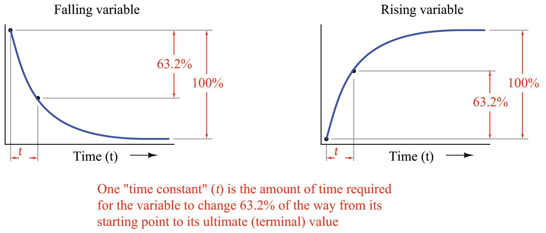
This mathematical analysis introduces a descriptive quantity of the system: something called a time constant. The “time constant” of a first-order system is the amount of time necessary for the system to come to within 36.8% (\(e^{-1}\)) of its final value (i.e. the time required for the system to go 63.2% of the way from the starting point to its ultimate settling point: \(1 - e^{-1}\)). After two time-constants’ worth of time, the system will have come to within 13.5% (\(e^{-2}\)) of its final value (i.e. gone 86.5% of the way: \(1 - e^{-2}\)); after three time-constants’ worth of time, to within 5% (\(e^{-3}\)) of the final value, (i.e. gone 95% of the way: \(1 - e^{-3}\)). After five time-constants’ worth of time, the system will be within 1% (\(e^{-5}\), rounded to the nearest whole percent) of its final value, which is often close enough to consider it “settled” for most practical purposes.
| Time | Percent of final value | Percent change remaining |
|---|---|---|
| 0 | 0.000\% | 100.000\% |
| $\tau$ | 63.212\% | 36.788\% |
| $2\tau$ | 86.466\% | 13.534\% |
| 3$\tau$ | 95.021\% | 4.979\% |
| 4$\tau$ | 98.168\% | 1.832\% |
| 5$\tau$ | 99.326\% | 0.674\% |
| 6$\tau$ | 99.752\% | 0.248\% |
| 7$\tau$ | 99.909\% | 0.091\% |
| 8$\tau$ | 99.966\% | 0.034\% |
| 9$\tau$ | 99.988\% | 0.012\% |
| 10$\tau$ | 99.995\% | 0.005\% |
The concept of a “time constant” may be shown in graphical form for both falling and rising variables:
Students of electronics will immediately recognize this concept, since it is widely used in the analysis and application of capacitive and inductive circuits. However, you should recognize the fact that the concept of a “time constant” for capacitive and inductive electrical circuits is only one case of a more general phenomenon. Literally any physical system described by the same first-order differential equation may be said to have a “time constant.” Thus, it is perfectly valid for us to speak of a hot cup of coffee as having a time constant (\(\tau\)), and to say that the coffee’s temperature will be within 1% of room temperature after five of those time constants have elapsed.
In the world of process control, it is more customary to refer to this as a lag time than as a time constant, but these are really interchangeable terms. The term “lag time” makes sense if we consider a first-order system driven to achieve a constant rate of change. For instance, if we subjected our RC circuit to a ramping input voltage rather than a “stepped” input voltage – such that the output ramped as well instead of passively settling at some final value – we would find that the amount of time separating equal input and output voltage values was equal to this time constant (in an RC circuit, \(\tau = RC\)):
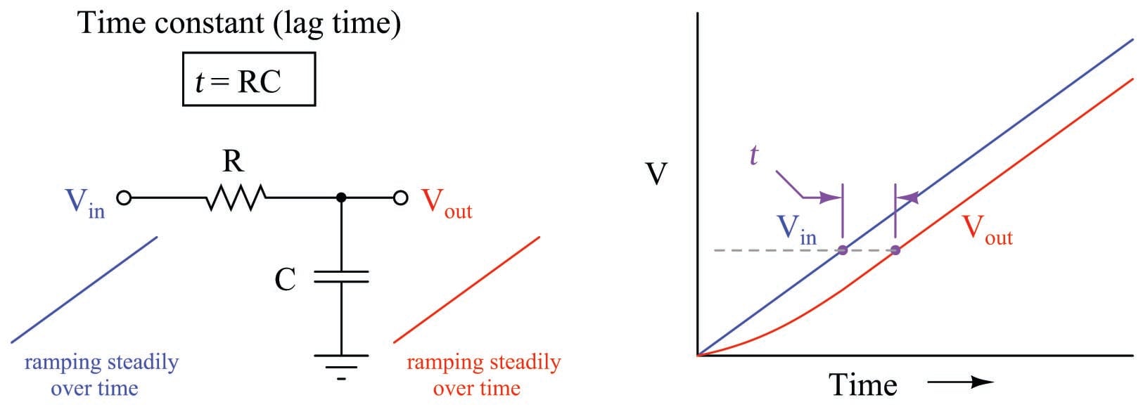
Lag time is thus defined as the difference in time between when the process variable ramps to a certain value and when it would have ramped to that same value were it not for the existence of first-order lag in the system. The system’s output variable lags behind the ramping input variable by a fixed amount of time, regardless of the ramping rate. If the process in question is an RC circuit, the lag time will still be the product of (\(\tau = RC\)), just as the “time product” defined for a stepped input voltage. Thus, we see that “time constant” and “lag time” are really the exact same concept, merely manifesting in different forms as the result of two different input conditions (stepped versus ramped).
When an engineer or a technician describes a process being “fast” or “slow,” they generally refer to the magnitude of this lag time. This makes lag time very important to our selection of PID controller tuning values. Integral and derivative control actions in particular are sensitive to the amount of lag time in a process, since both those actions are time-based. “Slow” processes (i.e. process types having large lag times) cannot tolerate aggressive integral action, where the controller “impatiently” winds the output up or down at a rate that is too rapid for the process to respond to. Derivative action, however, is generally useful on processes having large lag times.
Multiple lags (orders)
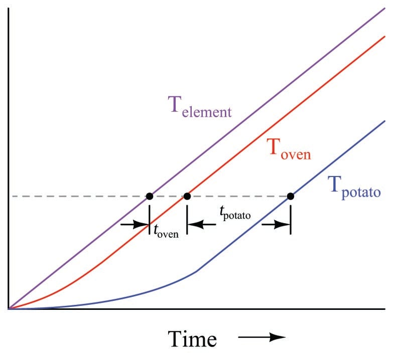
Simple, self-regulating processes tend to be first-order: that is, they have only one mechanism of lag. More complicated processes often consist of multiple sub-processes, each one with its own lag time. Take for example a convection oven, heating a potato. Being instrumentation specialists in addition to cooks, we decide to monitor both the oven temperature and the potato temperature using thermocouples and remote temperature indicators:
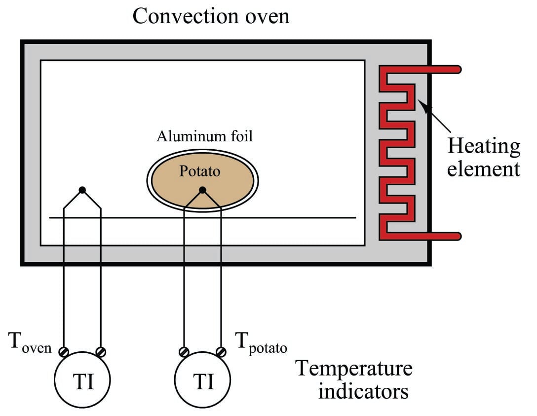
The oven itself is a first-order process. If we graph its temperature over time as the heater power is suddenly stepped up to some fixed value962, we will see a classic first-order response:
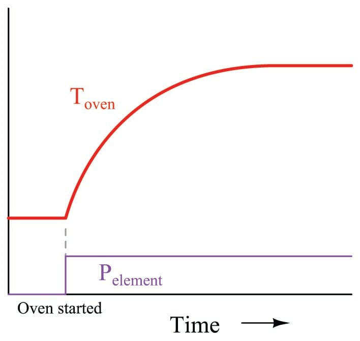
The potato forms another first-order process, absorbing heat from the air within the oven (heat transfer by convection), gradually warming up until its temperature (eventually) reaches that of the oven963. From the perspective of the heating element to the oven air temperature, we have a first-order process. From the perspective of the heating element to the potato, however, we have a second-order process.
Intuition might lead you to believe that a second-order process is just like a first-order process – except slower – but that intuition would be wrong. Cascading two first-order lags creates a fundamentally different time dynamic. In other words, two first-order lags do not simply result in a longer first-order lag, but rather a second-order lag with its own unique characteristics.
If we superimpose a graph of the potato temperature with a graph of the oven temperature (once again assuming constant power output from the heating element, with no thermostatic control), we will see that the shape of this second-order lag is different. The curve now has an “S” shape, rather than a consistent downward concavity:
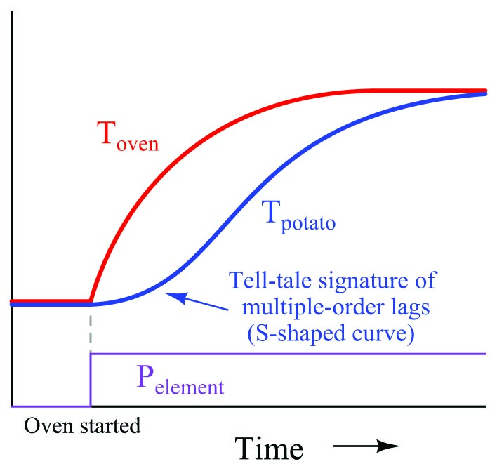
This, in fact, is one of the tell-tale signature of multiple lags in a process: an “S”-shaped curve rather than the characteristically abrupt initial rise of a first-order curve.
Another tell-tale signature of multiple lags is that the lagging variable does not immediately reverse its direction of change following a reversal in the final control element signal. We can see this effect by cutting power to the heating element before either the oven air or potato temperatures have reached their final values:
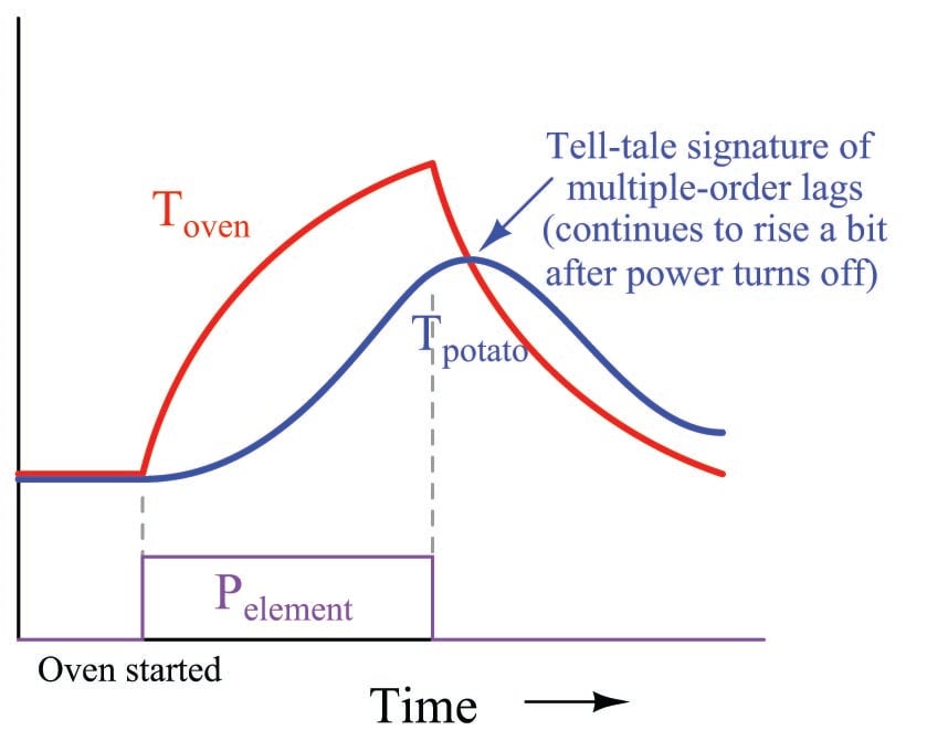
Note how the air temperature trend immediately reverses direction following the cessation of power to the heating element, but how the potato temperature trend continues to rise for a short amount of time964 before reversing direction and cooling. Here, the contrast between first-order and second-order lag responses is rather dramatic – the second-order response is clearly not just a longer version of the first-order response, but rather something quite distinct unto itself.
This is why multiple-order lag processes have a greater tendency to overshoot their setpoints while under automatic control: the process variable exhibits a sort of “inertia” whereby it fails to switch directions simultaneously with the controller output.
If we were able to ramp the heater power at a constant rate and graph the heater element, air, and potato temperatures, we would clearly see the separate lag times of the oven and the potato as offsets in time at any given temperature:
As another example, let us consider the control of level in three cascaded, gravity-drained vessels:
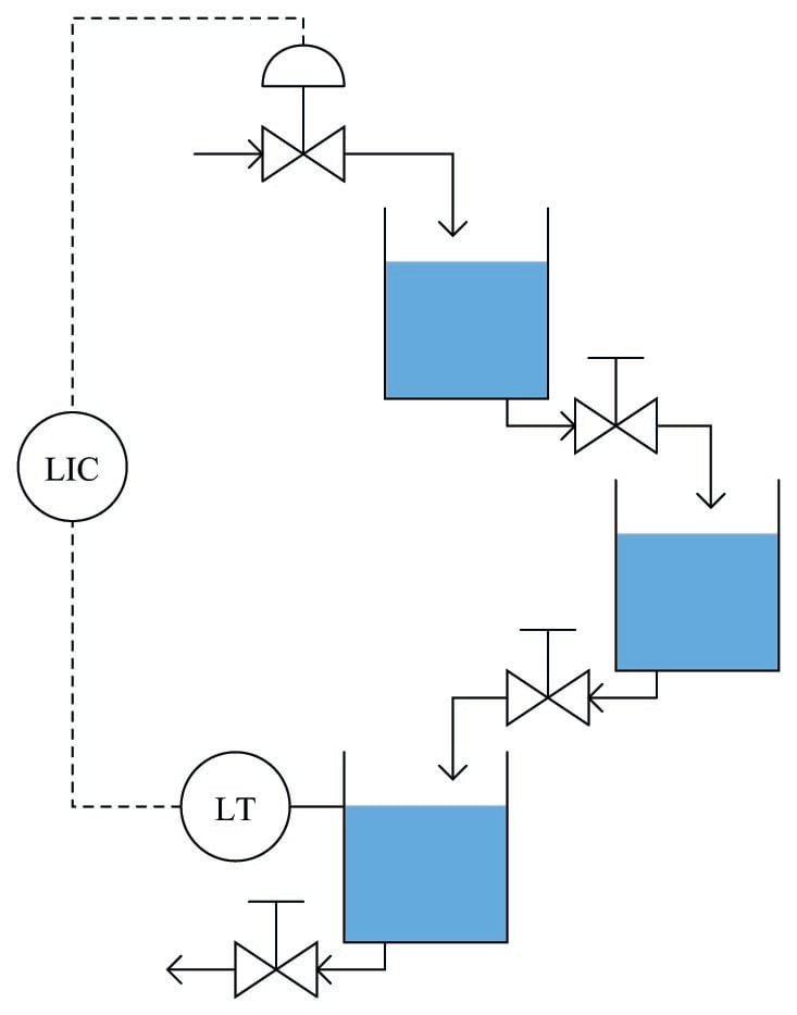
From the perspective of the level transmitter on the last vessel, the control valve is driving a third-order process, with three distinct lags cascaded in series. This would be a challenging process to control, and not just because of the possibility of the intermediate vessels overflowing (since their levels are not being measured)!
When we consider the dynamic response of a process, we are usually concerned primarily with the physical process itself. However, the instruments attached to that process also influence lag orders and lag times. As discussed in the previous subsection, almost every physical function exhibits some form of lag. Even the instruments we use to measure process variables have their own (usually very short) lag times. Control valves may have substantial lag times, measured in the tens of seconds for some large valves. Thus, a “slow” control valve exerting control over a first-order process effectively creates a second-order loop response. Thermowells used with temperature sensors such as thermocouples and RTDs can also introduce lag times into a loop (especially if the sensing element is not fully contacting the bottom of the well!).
This means it is nearly impossible to have a control loop with a purely first-order response. Many real loops come close to being first-order, but only because the lag time of the physical process swamps (dominates) the relatively tiny lag times of the instruments. For inherently fast processes such as liquid flow and liquid pressure control, however, the process response is so fast that even short time lags in valve positioners, transmitters, and other loop instruments significantly alter the loop’s dynamic character.
Multiple-order lags are relevant to the issue of PID loop tuning because they encourage oscillation. The more lags there are in a system, the more delayed and “detached” the process variable becomes from the controller’s output signal.
A system with lag time exhibits phase shift when driven by a sinusoidal stimulus: the outgoing waveform lags behind the input waveform by a certain number of degrees at one frequency. The exact amount of phase shift depends on frequency – the higher the frequency, the more phase shift (to a maximum of \(-90^{o}\) for a first-order lag):
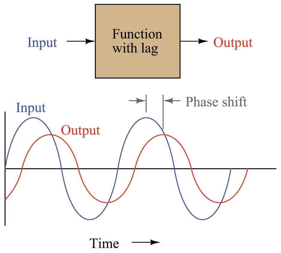
The phase shifts of multiple, cascaded lag functions (or processes, or physical effects) add up. This means each lag in a system contributes an additional negative phase shift to the loop. This can be detrimental to negative feedback, which by definition is a 180\(^{o}\) phase shift. If sufficient lags exist in a system, the total loop phase shift may approach 360\(^{o}\), in which case the feedback becomes positive (regenerative): a necessary965 condition for oscillation.
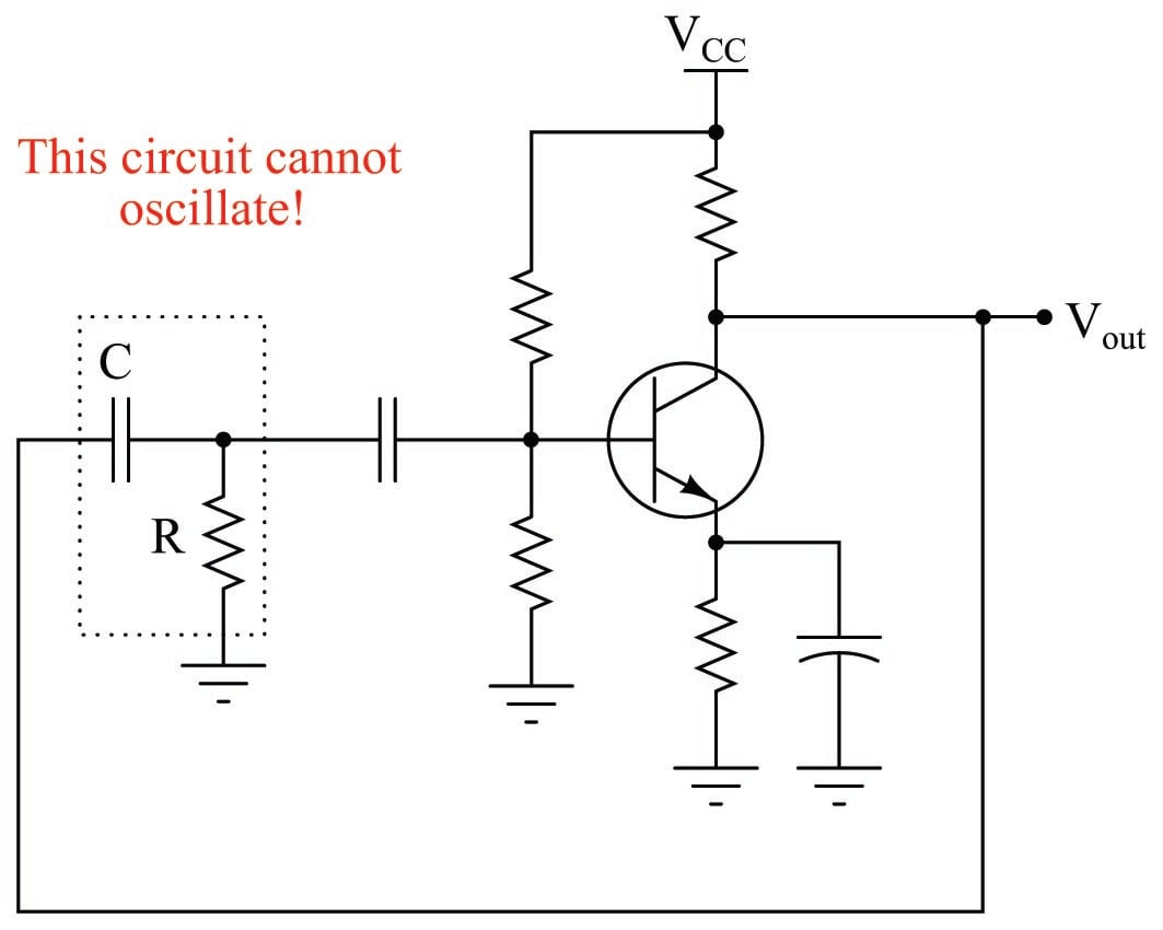
It is worthy to note that multiple-order lags are constructively applied in electronics when the express goal is to create oscillations. If a series of RC “lag” networks are used to feed the output of an inverting amplifier circuit back to its input with sufficient signal strength intact966, and those networks introduce another 180 degrees of phase shift, the total loop phase shift will be 360\(^{o}\) (i.e. positive feedback) and the circuit will self-oscillate. This is called an RC phase-shift oscillator circuit:
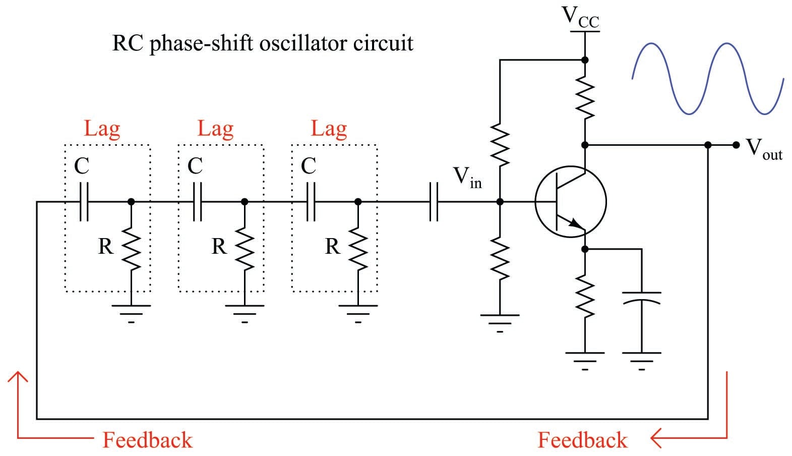
The amplifier works just like a proportional-only process controller, with action set for negative feedback. The resistor-capacitor networks act like the lags inherent to the process being controlled. Given enough controller (amplifier) gain, the cascaded lags in the process (RC networks) create the perfect conditions for self-oscillation. The amplifier creates the first 180\(^{o}\) of phase shift (being inverting in nature), while the RC networks collectively create the other 180\(^{o}\) of phase shift to give a total phase shift of 360\(^{o}\) (positive, or regenerative feedback).
In theory, the most phase shift a single RC network can create is \(-90^{o}\), but even that is not practical967. This is why more than two RC phase-shifting networks are required for successful operation of an RC phase-shift oscillator circuit.
As an illustration of this point, the following circuit is incapable968 of self-oscillation. Its lone RC phase-shifting network cannot create the -180\(^{o}\) phase shift necessary for the overall loop to have positive feedback and oscillate:
The RC phase-shift oscillator circuit design thus holds a very important lesson for us in PID loop tuning. It clearly illustrates how multiple orders of lag are a more significant obstacle to robust control than a single lag time of any magnitude. A purely first-order process will tolerate enormous amounts of controller gain without ever breaking into oscillations, because it lacks the phase shift necessary to self-oscillate. This means – barring any other condition limiting our use of high gain, such as process noise – we may use very aggressive proportional-only action (e.g. gain values of 20 or more) to achieve robust control on a first-order process969. Multiple-order processes are less forgiving of high controller gains, because they are capable of generating enough phase shift to self-oscillate.
Dead time
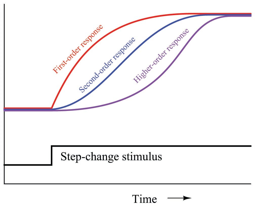
Lag time refers to a damped response from a process, from a change in manipulated variable (e.g. control valve position) to a measured change in process variable: the initial effect of a change in controller output is immediately seen, but the final effect takes time to develop. Dead time, by contrast, refers to a period of time during which a change in manipulated variable produces no effect whatsoever in the process variable: the process appears “dead” for some amount of time before showing a response. The following graph contrasts first-order and multiple-order lag times against pure dead time, as revealed in response to a manual step-change in the controller’s output (an “open-loop” test of the process characteristics):
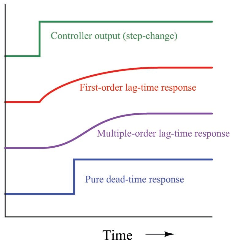
Although the first-order response does takes some time to settle at a stable value, there is no time delay between when the output steps up and the first-order response begins to rise. The same may be said for the multiple-order response, albeit with a slower rate of initial rise. The dead-time response, however, is actually delayed some time after the output makes its step-change. There is a period of time where the dead-time response does absolutely nothing following the output step-change.
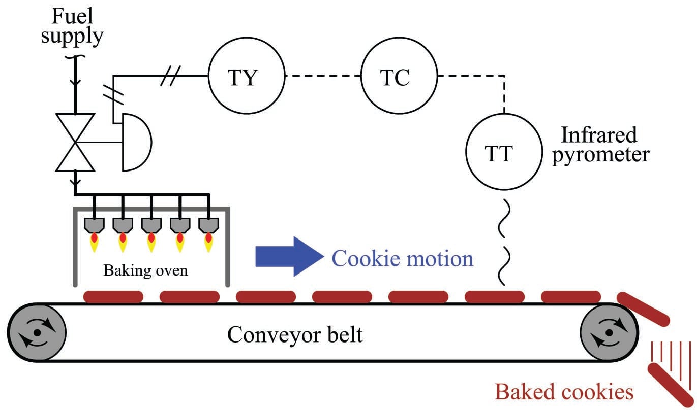
Dead time is also referred to as transport delay, because the mechanism of dead time is often a time delay caused by the transportation of material at finite speed across some distance. The following cookie-baking process has dead time by virtue of the time delay inherent to the cookies’ journey from the oven to the temperature sensor:
Dead time is a far worse problem for feedback control systems than lag time. The reason why is best understood from the perspective of phase shift: the delay (measured in degrees of angular displacement) between input and output for a system driven by a sinusoidal stimulus. Excessive phase shift in a feedback system makes possible self-sustaining oscillations, turning what is supposed to be negative feedback into positive feedback. Systems with lag produce phase shift that is frequency-dependent (the greater the frequency, the more the output “lags” behind the input), but this phase shift has a natural limit. For a first-order lag function, the phase shift has an absolute maximum value of \(-90^{o}\); second-order lag functions have a theoretical maximum phase shift of \(-180^{o}\); and so on. Dead time functions also produce phase shift that increases with frequency, but there is no ultimate limit to the amount of phase shift. This means a single dead-time element in a feedback control loop is capable of producing any amount of phase shift given the right frequency970. What is more, the gain of a dead time function usually does not diminish with frequency, unlike the gain of a lag function.
Recall that a feedback system will self-oscillate if two conditions are met: a total phase shift of 360\(^{o}\) (or \(-360^{o}\): the same thing) and a total loop gain of at least one. Any feedback system meeting these criteria971 will oscillate, be it an electronic amplifier circuit or a process control loop. In the interest of achieving robust process control, we need to prevent these conditions from ever occurring simultaneously.
A visual comparison between the phase shifts and gains exhibited by lag versus dead time functions may be seen here, the respective functions modeled by the electrical entities of a simple RC network (lag time) and an LC “delay line” network (dead time):
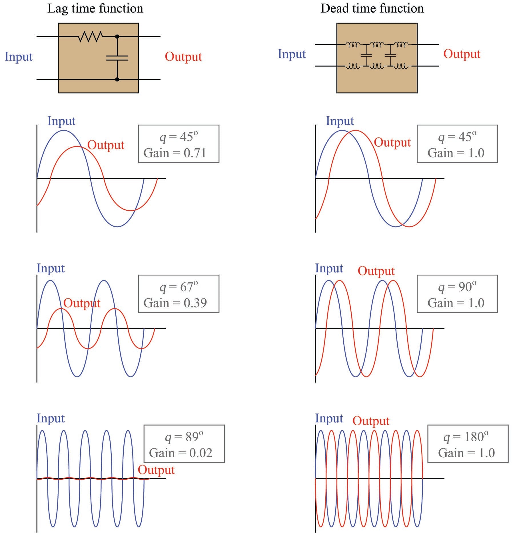
As frequency increases, the lag time function’s phase shift asymptotically approaches \(-90^{o}\) while its attenuation asymptotically approaches zero. Ultimately, when the phase shift reaches its maximum of \(-90^{o}\), the output signal amplitude is reduced to nothing. By contrast, the dead time function’s phase shift grows linearly with frequency (to \(-180^{o}\) and beyond!) while its attenuation remains unchanged. Clearly, dead time better fulfills the dual criteria of sufficient phase shift and sufficient loop gain needed for feedback oscillation than lag time, which is why dead time invites oscillation in a control loop more than lag time.
Pure dead-time processes are rare. Usually, an industrial process will exhibit at least some degree of lag time in addition to dead time. As strange as it may sound, this is a fortunate for the purpose of feedback control. The presence of lag(s) in a process guarantees a degradation of loop gain with frequency increase, which may help avoid oscillation. The greater the ratio between dead time and lag time in a loop, the more unstable it tends to be.
The appearance of dead time may be created in a process by the cascaded effect of multiple lags. As mentioned in an earlier subsection, multiple lags create a process response to step-changes that is “S”-shaped, responding gradually at first instead of immediately following the step-change. Given enough lags acting in series, the beginning of this “S” curve may be so flat that it appears “dead:”
While dead time may be impossible to eliminate in some processes, it should be minimized wherever possible due to its detrimental impact on feedback control. Once an open-loop (manual-mode step-change) test on a process confirms the existence of dead time, the source of dead time should be identified and eliminated if at all possible.
One technique applied to the control of dead-time-dominant processes is a special variation of the PID algorithm called sample-and-hold. In this variation of PID, the controller effectively alternates between “automatic” and “manual” modes according to a pre-programmed cycle. For a short period of time, it switches to “automatic” mode in order to “sample” the error (PV \(-\) SP) and calculate a new output value, but then switches right back into “manual” mode (“hold”) so as to give time for the effects of those corrections to propagate through the process dead time before taking another sample and calculating another output value. This sample-and-hold cycle of course slows the controller’s response to changes such as setpoint adjustments and load variations, but it does allow for more aggressive PID tuning constants than would otherwise work in a continuously sampling controller because it effectively blinds972 the controller from “seeing” the time delays inherent to the process.
All digital instruments exhibit dead time due to the nature of their operation: processing signals over discrete time periods. Usually, the amount of dead time seen in a modern digital instrument is too short to be of any consequence, but there are some special cases meriting attention. Perhaps the most serious case is the example of wireless transmitters, using radio waves to communicate process information back to a host system. In order to maximize battery life, a wireless transmitter must transmit its data sparingly. Update times (i.e. dead time) measured in minutes are not uncommon for battery-powered wireless process transmitters.
Hysteresis
A detrimental effect to feedback control is a characteristic known as hysteresis: a lack of responsiveness to a change in direction. Although hysteresis typically resides with instruments rather than the physical process they connect to, it is most easily detected by a simple open-loop (“step-change”) test with the controller in manual mode just like all the important process characteristics (self-regulating versus integrating, steady-state gain, lag time, dead time, etc.).
The most common source of hysteresis is found in pneumatically-actuated control valves possessing excess stem friction. The “jerky” motion of such a valve to smooth increases or decreases in signal is sometimes referred to as stiction. Similarly, a pneumatically-actuated control valve with excess friction will be unresponsive to small reversals in signal direction. To illustrate, this means the control valve’s stem position will not be the same at a rising signal value of 50% (typically 12 mA, or 9 PSI) as it will be at a falling signal value of 50%.
Control valve stiction may be quite severe in valves with poor maintenance histories, and/or lacking positioners to correct for deviations between controller signal value and actual stem position. I have personally encountered control valves with hysteresis values in excess of 10%973, and have heard of even more severe cases.
Detecting hysteresis in a control loop is as simple as performing “up-and-down” tests of the controller output signal in manual mode. The following trend shows how hysteresis might appear in a self-regulating process such as liquid flow control:
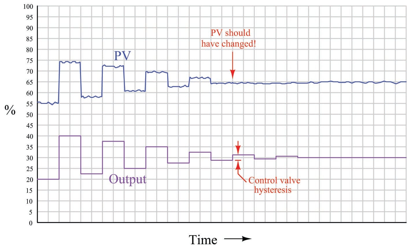
Note how the PV responds to large up-and-down output step-changes, but stops responding as soon as the magnitude of these open-loop step-changes falls below a threshold equal to the control valve’s hysteresis.
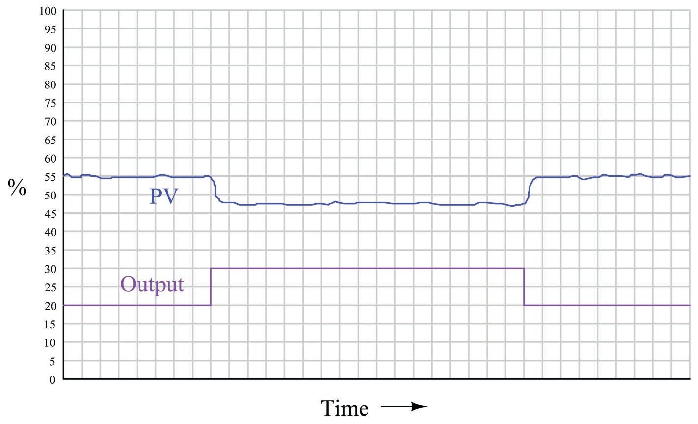
Applied to an integrating process such as liquid level control, the same type of test reveals the control valve’s hysteresis by the largest step-change that does not alter the PV’s slope:
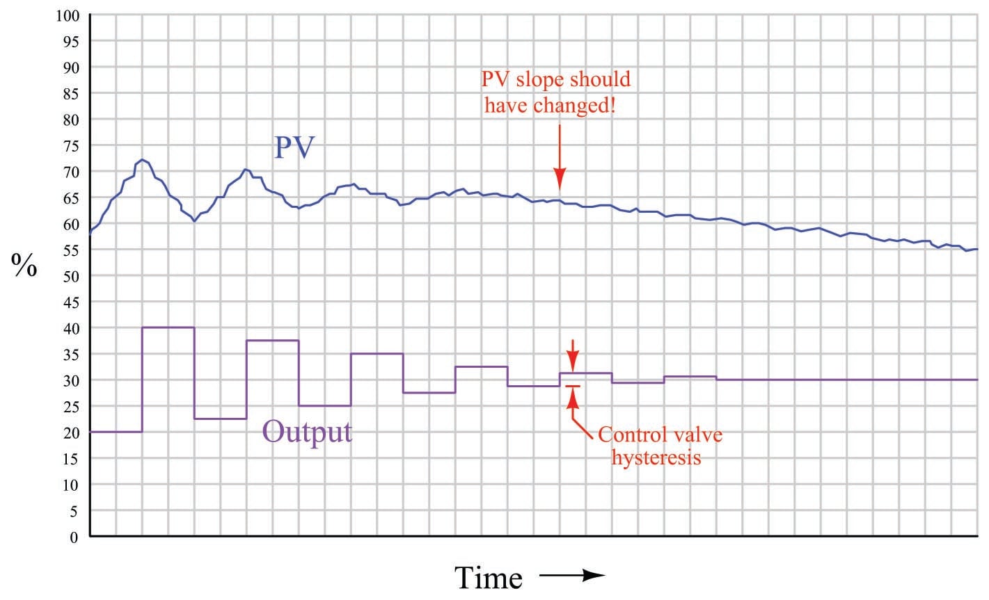
It is not as simple to perform this test on a process with slow lag or dead times, of course, or on a process possessing a “runaway” (rather than self-regulating or integrating) characteristic, in which case a better test for valve hysteresis would be to monitor valve stem position rather than the PV when executing the step-changes.
Hysteresis is a problem in feedback control because it essentially acts like a variable dead time. Recall that “dead time” was defined as a period of time during which a change in manipulated variable produces no effect in the process variable: the process appears “dead” for some amount of time before showing a response. If a change in controller output (manipulated variable) is insufficient to overcome the hysteresis inherent to a control valve or other component in a loop, the process variable will not respond to that output signal change at all. Only when the manipulated variable signal continues to change sufficiently to overcome hysteresis will there be a response from the process variable, and the time required for that to take place depends on how soon the controller’s output happens to reach that critical value. If the controller’s output moves quickly, the “dead time” caused by hysteresis will be short. If the controller’s output changes slowly over time, the “dead time” caused by hysteresis will be longer.
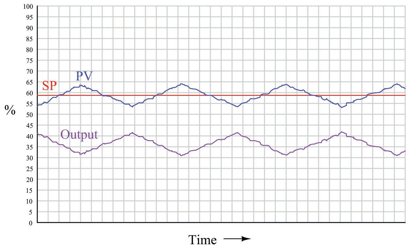
Another problem caused by hysteresis in a feedback loop occurs in combination with integral action, whether it be programmed into the controller or is inherent to the process (i.e. an integrating process). It is highly unlikely that a “sticky” control valve will happen to “stick” at exactly the right stem position required to equalize PV and SP. Therefore, the probability at any time of an error developing between PV and SP, or of an offset developing between the valve position and the equilibrium position required by an integrating process, is very great. This leads to a condition of guaranteed instability. For a self-regulating process with integral action in the controller, the almost guaranteed existence of PV \(-\) SP error means the controller output will ceaselessly ramp up and down as the valve first slips and sticks to give a positive error, then slips and sticks to give a negative error. For an integrating process with proportional action in the controller, the process variable will ceaselessly ramp up and down as the valve first sticks too far open, then too far closed to equalize process in-flow and out-flow which is necessary to stabilize the process variable. In either case, this particular form of instability is called a slip-stick cycle.
The following process trend shows a slip-stick cycle in a self-regulating process, controlled by an integral-only controller:
Note how the output ceaselessly ramps in a futile attempt to drive the process variable to setpoint. Once sufficient pressure change accumulates in the valve actuator to overcome static stem friction, the valve “slips to and sticks at” a new stem position where the PV is unequal to setpoint, and the controller’s integral action begins to ramp the output in the other direction.
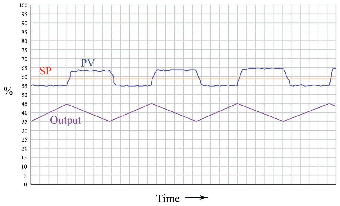
The next trend shows a slip-stick cycle in an integrating process, controlled by a proportional-only controller:
Note how the process variable’s slope changes every time the valve “slips to and sticks at” a new stem position unequal to the balance point for this integrating process. The process’s natural integrating action then causes the PV to ramp, causing the controller’s proportional action to similarly ramp the output signal until the valve has enough accumulated force on its stem to jump to a new position.
It is very important to note that the problems created by a “sticky” control valve cannot be completely overcome by controller tuning974. For instance, if one were to de-tune the integral-only controller (i.e. longer time constant, or fewer repeats per minute) in the self-regulating process, it would still exhibit the same slip-stick behavior, only over a longer period (lower frequency) than before. If one were to de-tune the proportional-only controller (i.e. greater proportional band, or less gain) in the integrating process, the exact same thing would happen: a decrease in cycle frequency, but no elimination of the cycling. Furthermore, de-tuning the controller in either process would also result in less responsive (poorer) corrective action to setpoint and load changes. The only solution975 to either one of these problems is to reduce or eliminate the friction inside the control valve.

very informing