 Facebook
 Google
 GitHub
 Linkedin
Tuning PID Controllers
Learning how to tune PID controllers is a skill born of much practice. Regardless of how thoroughly you may study the subject of PID control on paper, you really do not understand it until you have spent a fair amount of time actually tuning real controllers.
In order to gain this experience, though, you need access to working processes and the freedom to disturb those processes over and over again. If your school’s lab has several “toy” processes built to facilitate this type of learning experience, that is great. However, your learning will grow even more if you have a way to practice PID tuning at your own convenience.
Electrically simulating a process
Thankfully, there is a relatively simple way to build your own “process” for PID tuning practice. First, you need to obtain an electronic single-loop PID controller990 and connect it to a resistor-capacitor network such as this:
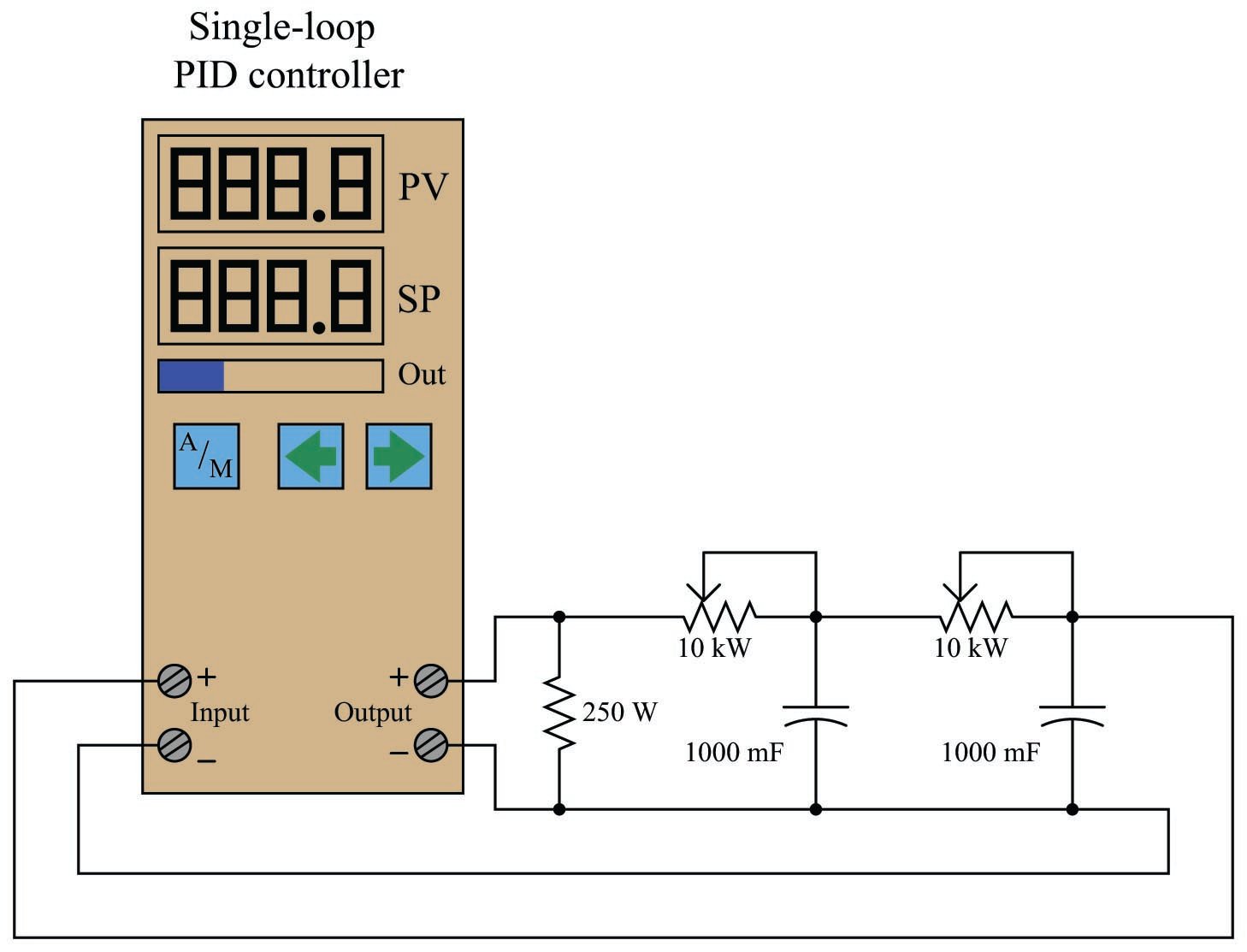
The 250 \(\Omega\) resistor converts the controller’s 4-20 mA signal into a 1-5 VDC signal, which then drives the passive integrator (lag) RC networks. The two stages of RC “lag” simulate a self-regulating process with a second-order lag and a steady-state gain of 1. The potentiometers establish the lag times for each stage, providing a convenient way to alter the process characteristics for more tuning practice. Feel free to extend the circuit with additional RC lag networks for even more delay (and an even harder-to-tune process!).
Since this simulated “process” is direct-acting (i.e. increasing manipulated variable signal results in an increasing process variable signal), the controller must be configured for reverse action (i.e. increasing process variable signal results in a decreasing manipulated variable signal) in order to achieve negative feedback. You are welcome to configure the controller for direct action just to see what the effects will be, but I assure you control will be impossible: the PV will saturate beyond 100% or below 0% no matter how the PID values are set.
Building a “Desktop Process” unit
A more sophisticated approach to gaining hands-on experience tuning PID controllers is to actually build a working “process” that the controller can regulate. A relatively simple way to do this for students is to build what I like to call Desktop Processes, where a loop controller is used to control the speed of a motor/generator set made from small DC “hobby” electric motors. An illustration of a “Desktop Process” is shown here:
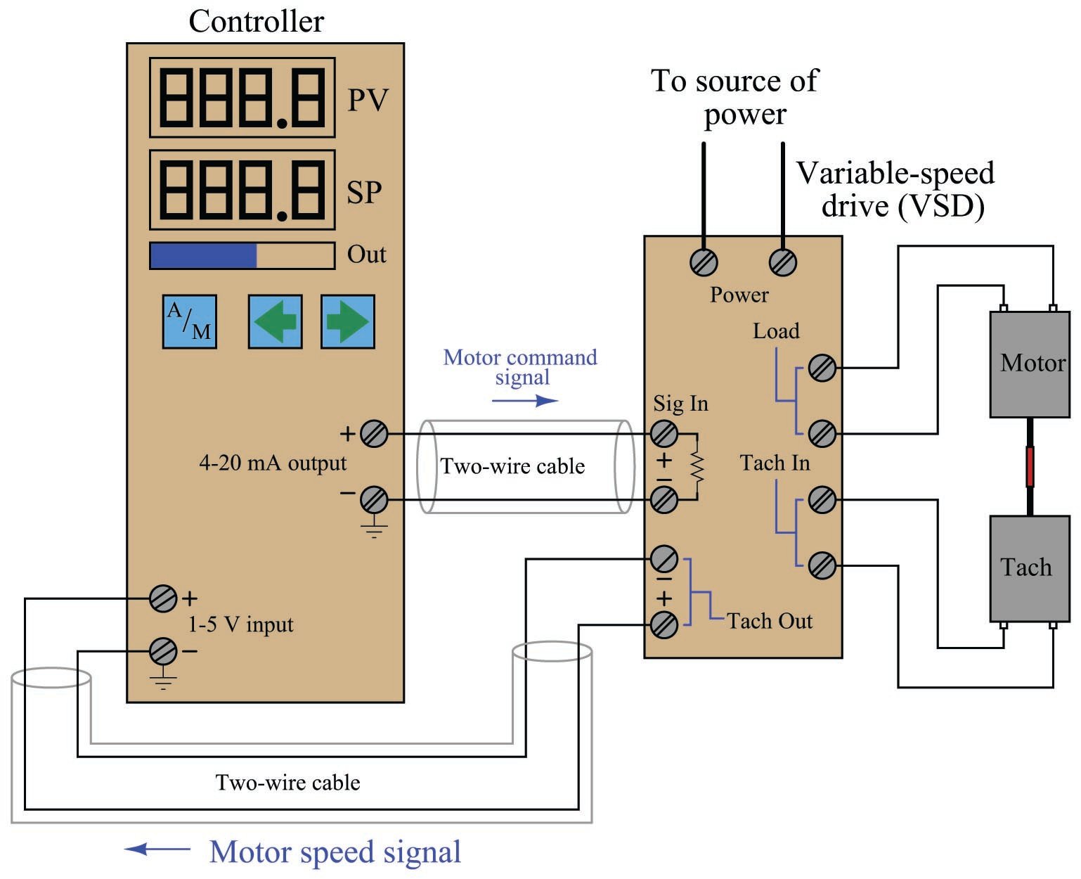
You must build your own variable-speed drive (VSD) circuit to convert the controller’s 4-20 mA output signal into a DC voltage powerful enough to drive the motor. This same circuit should also contain components for “scaling” and filtering the tachogenerator’s DC voltage signal so it may be read by the controller’s input. Fortunately, the following circuit is a proven and simple design for doing just that:
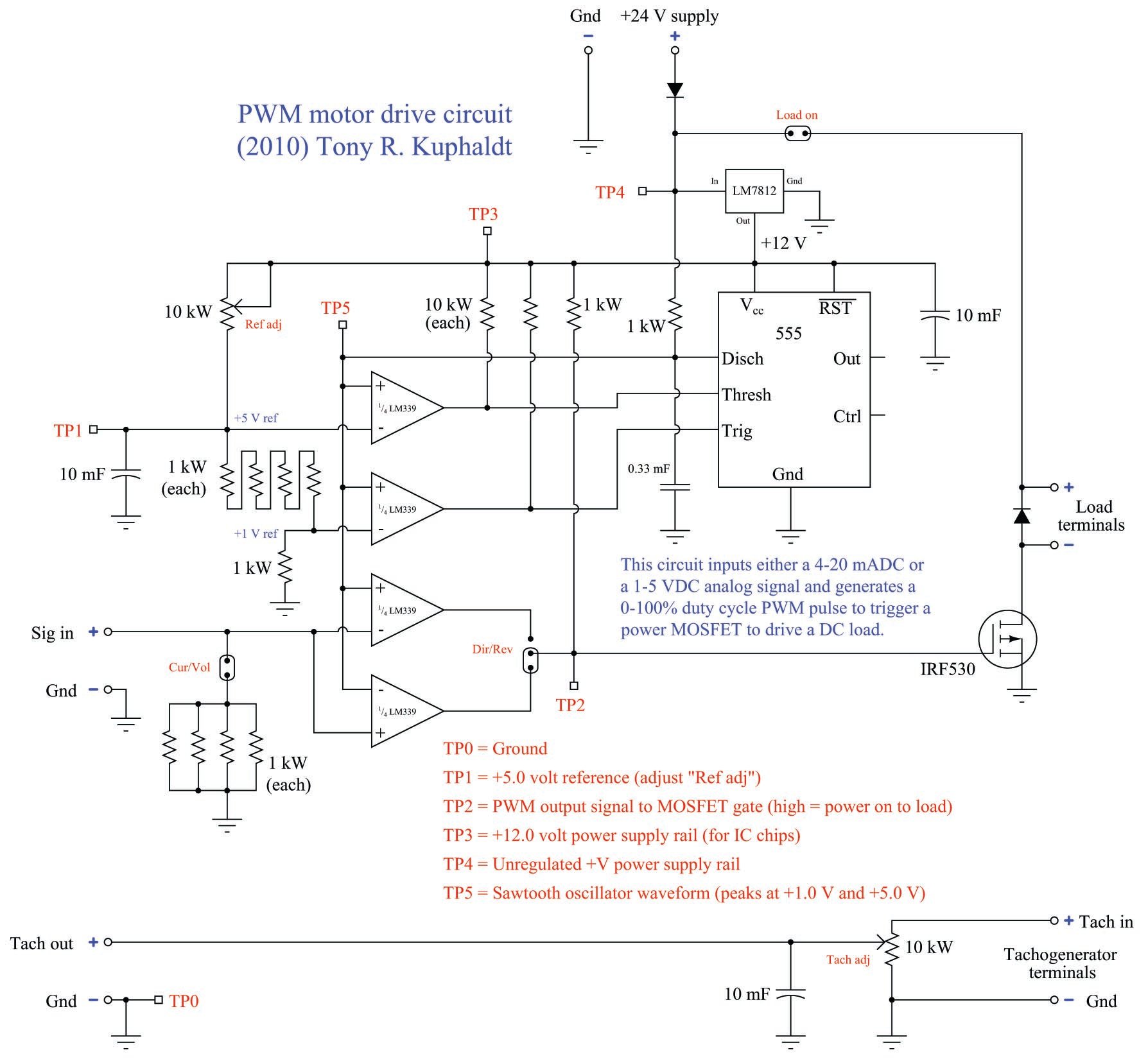
Diodes included in this design protect against reverse-polarity power supply connections and inductive “kickback” resulting from de-energizing inductive loads.
Photographs showing a complete “Desktop Process” unit in operation, including close-ups of the motor/generator set and the variable speed drive circuit board, appear here:
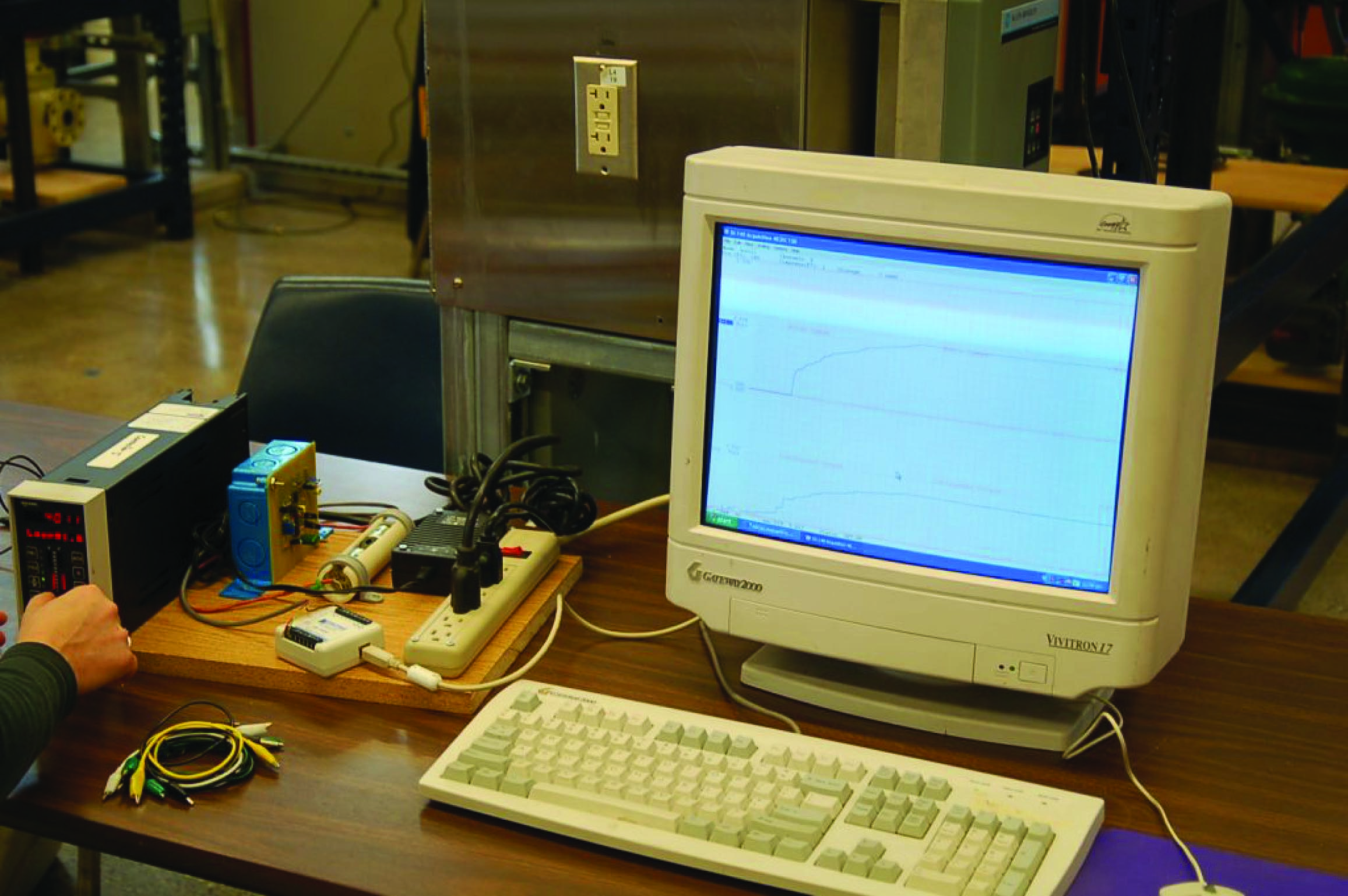
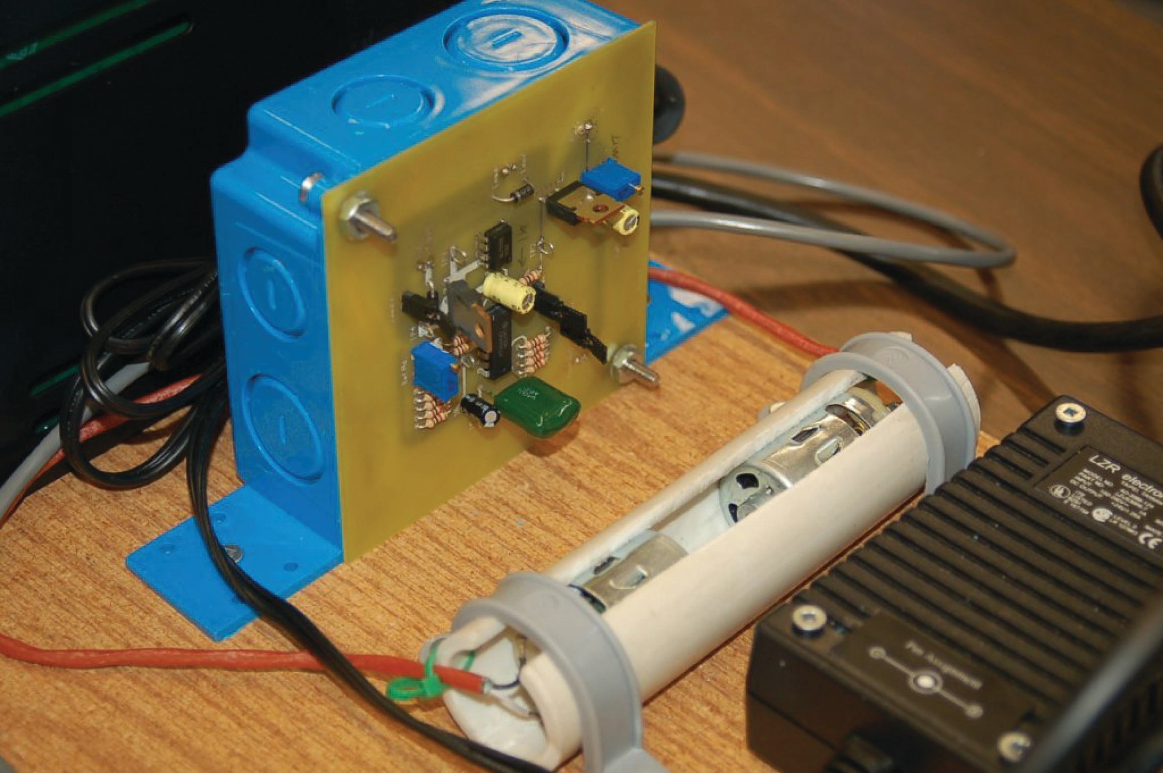
As you can see from the photograph, the motor and generator are held in a short length of split PVC pipe. This is a simple way to clamp and align both machines so their shafts turn on the same centerline. The coupling between the two shafts is nothing more than a piece of rubber tube (or wire insulation, or heat-shrink tubing, or even electrical tape!).
An optional accessory to add to a Desktop Process is a data acquisition unit capable of measuring the DC voltage motor speed and controller output signals, plotting them on a computer display for further analysis. This becomes very useful when fine-tuning PID response, allowing students to visually recognize oscillation, overshoot, windup, and other phenomena of closed-loop control.
The controller model shown in these photographs happens to be a Siemens 353, but any loop controller capable of receiving a 1-5 volt DC input signal and generating 4-20 mA DC output signal will work just fine. In fact, I’ve connected this very same VSD and motor/generator set to different controllers991 to compare operation.
Interesting experiments to perform with a Desktop Process – other than PID tuning practice – include the following:
- Introducing process loads by touching the spinning motor shaft (slowing it down using your finger) and compare the responses between the controller’s “manual” and “automatic” modes. This proves to be a very effective way for students to comprehend the difference between these two modes of operation. I have yet to encounter a student who does not immediately grasp the concept after doing this experiment for themselves, feeling the motor’s shaft speed respond to their finger load in both modes, also watching the controller’s output response.
- Switching the controller mode from reverse action to direct action to see how a process “runs away” when the loop feedback is positive rather than negative.
- Switching the VSD action from direct to reverse, then reconfiguring the controller’s action to complement it, maintaining negative feedback in the system.
- Try switching between auto and manual modes in the controller, comparing the response with and without the feature of setpoint tracking. Again, this is a concept many students struggle to grasp in theory, but immediately comprehend when they see it in action.
Simulating a process by computer
A fascinating solution for realistic PID tuning in the classroom was offered to me by Blair MacNeil of Cape Breton University (located in the town of Sydney, on the island of Nova Scotia, Canada) in 2010 by way of email correspondence. Professor MacNeil uses Moore 353 loop controllers connected to analog computer I/O (“data acquisition”) modules, with a personal computer running VisSim Realtime software to simulate the dynamics of a real process. With the power of a personal computer simulating the process, virtually any process dynamic (as well as any instrument fault) may be generated for the benefit of the loop controller to control:
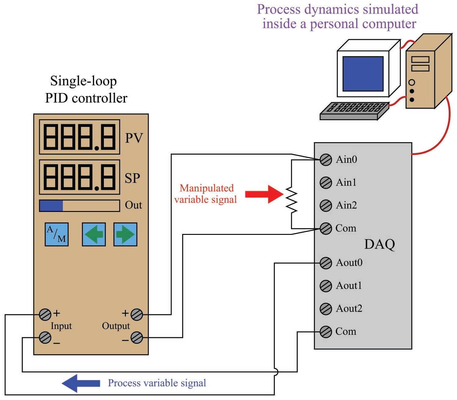
This approach provides realistic process dynamics for the loop controller to manage, yet requires little in the way of capital expense or physical space to implement. Different process models, instrument faults, and control strategies may be easily implemented in the personal computer’s software, making it far more flexible as a teaching tool than any analog electronic simulation network or real process connected to the controller. It is also completely safe to operate, with absolutely no danger of harming anything in the event of a process “excursion” or other upset.
