 Facebook
 Google
 GitHub
 Linkedin
Vibration Physics
One very convenient feature of waves is that their properties are universal. Waves of water in the ocean, sound waves in air, electronic signal waveforms, and even waves of mechanical vibration may all be expressed in mathematical form using the trigonometric sine and cosine functions. This means the same tools (both mathematical and technological) may be applied to the analysis of different kinds of waves. A strong example of this is the Fourier Transform, used to determine the frequency spectrum of a waveform, which may be applied with equal validity to any kind of wave.
Sinusoidal Vibrations
If a rotating wheel is unbalanced by the presence of an off-center mass, the resulting vibration will take the form of a cosine wave as measured by a displacement (position) sensor near the periphery of the object (assuming an angle of zero is defined by the position of the displacement sensor). The displacement sensor measures the air gap between the sensor tip and the rim of the spinning wheel, generating an electronic signal (most likely a voltage) directly proportional to that gap:
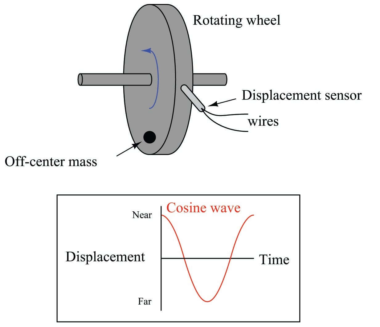
Since the wheel’s shaft “bows” in the direction of the off-center mass as it spins, the gap between the wheel and the sensor will be at a minimum at 0\(^{o}\), and maximum at 180\(^{o}\).
We may begin to express this phenomenon mathematically using the cosine function:
\[x = D \cos \omega t + b\]
Where,
\(x\) = Displacement as measured by sensor at time \(t\)
\(D\) = Peak displacement amplitude
\(\omega\) = Angular velocity (typically expressed in units of radians per second)
\(b\) = “Bias” air gap measured with no vibration
\(t\) = Time (seconds)
Since the cosine function alternates between extreme values of +1 and \(-1\), the constant \(D\) is necessary in the formula as a coefficient relating the cosine function to peak displacement. The cosine function’s argument (i.e. the angle given to it) deserves some explanation as well: the product \(\omega t\) is the multiple of angular velocity and time, angular velocity typically measured in radians per second and time typically measured in seconds. The product \(\omega t\), then, has a unit of radians. At time=0 (when the mass is aligned with the sensor), the product \(\omega t\) is zero and the cosine’s value is +1.
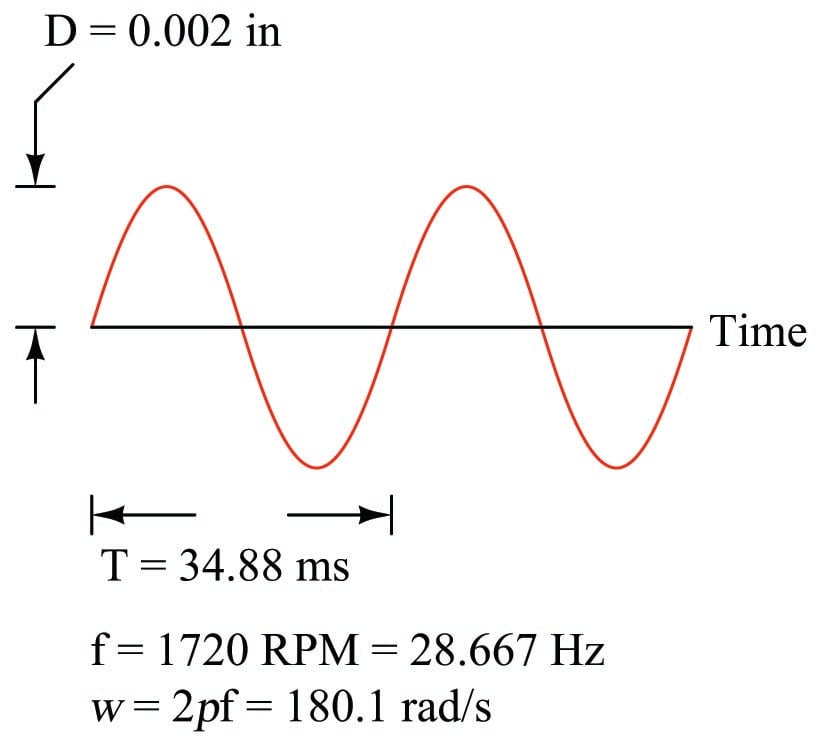
For a wheel spinning at 1720 RPM (approximately 180.1 radians per second), the angle between the off-center mass and the sensor will be as follows:
| Time | Angle (radians) | Angle (deg) | Angle (\(\cos \omega t\)) |
|---|---|---|---|
| 0 ms | 0 rad | 0\(^{o}\) | +1 |
| 8.721 ms | \(\pi \over 2\) rad | 90\(^{o}\) | 0 |
| 17.44 ms | \(\pi\) rad | 180\(^{o}\) | -1 |
| 26.16 ms | \(3 \pi \over 2\) rad | 270\(^{o}\) | 0 |
| 34.88 ms | 0 rad | 360\(^{o}\) or 0\(^{o}\) | +1 |
We know from physics that velocity is the time-derivative of displacement. That is, velocity is defined as the rate at which displacement changes over time. Mathematically, we may express this relationship using the calculus notation of the derivative:
\[v = {dx \over dt} \hspace{30pt} or \hspace{30pt} v = {d \over dt}(x)\]
Where,
\(v\) = Velocity of an object
\(x\) = Displacement (position) of an object
\(t\) = Time
Since we happen to know the equation describing displacement (\(x\)) in this system, we may differentiate this equation to arrive at an equation for velocity:
\[v = {dx \over dt} = {d \over dt} (D \cos \omega t + b)\]
Applying the differentiation rule that the derivative of a sum is the sum of the derivatives:
\[v = {d \over dt} (D \cos \omega t) + {d \over dt} b\]
Recall that \(D\), \(\omega\), and \(b\) are all constants in this equation. The only variable here is \(t\), which we are differentiating with respect to. We know from calculus that the derivative of a simple cosine function is a negative sine (\({d \over dx} \cos x = -\sin x\)), and that the presence of a constant multiplier in the cosine’s argument results in that multiplier applied to the entire derivative (\({d \over dx} \cos ax = -a \sin ax\)). We also know that the derivative of any constant is simply zero (\({d \over dx} C = 0\)), which eliminates the \(b\) term:
\[v = -\omega D \sin \omega t\]
What this equation tells us is that for any given amount of peak displacement (\(D\)), the velocity of the wheel’s “wobble” increases linearly with speed (\(\omega\)). This should not surprise us, since we know an increase in rotational speed would mean the wheel displaces the same vibrating distance in less time, which would necessitate a higher velocity of vibration.
We may take the process one step further by differentiating the equation again with respect to time in order to arrive at an equation describing the vibrational acceleration of the wheel’s rim, since we know acceleration is the time-derivative of velocity (\(a = {dv \over dt}\)):
\[a = {dv \over dt} = {d \over dt} (-\omega D \sin \omega t)\]
From calculus, we know that the derivative of a sine function is a cosine function (\({d \over dx} \sin x = \cos x\)), and the same rule regarding constant multipliers in the function’s argument applies here as well (\({d \over dx} \sin ax = a \cos ax\)):
\[a = -\omega^2 D \cos \omega t\]
What this equation tells us is that for any given amount of peak displacement (\(D\)), the acceleration of the wheel’s “wobble” increases with the square of the speed (\(\omega\)). This is of great importance to us, since we know the lateral force imparted to the wheel (and shaft) is proportional to the lateral acceleration and also the mass of the wheel, from Newton’s Second Law of Motion:
\[F = ma\]
Therefore, the vibrational force experienced by this wheel grows rapidly as rotational speed increases:
\[F = ma = -m \omega^2 D \cos \omega t\]
This is why vibration can be so terribly destructive to high-speed rotating machinery. Even a small amount of lateral displacement caused by a mass imbalance or other effect may generate enormous forces on the rotating part(s), as these forces grow with the square of the rotating speed (e.g. doubling the speed quadruples the force; tripling the speed increases force by 9 times). Worse yet, these proportions assume a constant displacement (\(D\)), which is a best-case scenario. More realistically, we may expect the displacement to actually increase, as the centrifugal force generated by the off-center mass bends the rotating shaft to place the mass even farther away from the shaft centerline. Thus, doubling or tripling an imbalanced machine’s speed may multiply vibrational forces well in excess of four or nine times, respectively.
In the United States, it is customary to measure vibrational displacement (\(D\)) in units of mils, with one “mil” being \(1 \over 1000\) of an inch (0.001 inch). Vibrational velocity is measured in inches per second, following the displacement unit of the inch. Acceleration, although it could be expressed in units of inches per second squared, is more often represented in the unit of the G: a multiple of Earth’s own gravitational acceleration.
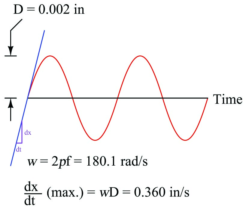
To give perspective to these units, it is helpful to consider a real application. Suppose we have a rotating machine vibrating in a sinusoidal (sine- or cosine-shaped) manner with a peak displacement (\(D\)) of 2 mils (0.002 inch) at a rotating speed of 1720 RPM (revolutions per minute). The frequency of this rotation is 28.667 Hz (revolutions per second), or 180.1 radians per second:
If \(D\) is the peak displacement of the sinusoid, then \(\omega D\) must be the peak velocity (maximum rate-of-change over time) of the sinusoid. This yields a peak velocity of 0.360 inches per second:
We may apply differentiation once more to obtain the acceleration of this machine’s rotating element. If \(D\) is the peak displacement of the sinusoid, and \(\omega D\) the peak velocity, then \(\omega^2 D\) will be its peak acceleration.
\[D = \hbox{Peak displacement} = 0.002 \hbox{ in}\]
\[\omega D = \hbox{Peak velocity} = 0.360 \hbox{ in/s}\]
\[\omega^2 D = \hbox{Peak acceleration} = 64.9 \hbox{ in/s}^2\]
The average value of Earth’s gravitational acceleration (\(g\)) is 32.17 feet per second squared. This equates to about 386 inches per second squared. Since our machine’s peak vibrational acceleration is 64.9 inches per second squared, this may be expressed as a “G” ratio to Earth’s gravity:
\[{{64.9 \hbox{ in/s}^2} \over {386 \hbox{ in/s}^2}} = 0.168 \hbox{ G's of peak acceleration}\]
Using “G’s” as a unit of acceleration makes it very easy to calculate forces imparted to the rotating element. If the machine’s rotating piece weighs 1200 pounds (in 1 “G” of Earth gravity), then the force imparted to this piece by the vibrational acceleration of 0.168 G’s will be 16.8% of its weight, or 201.7 pounds.
Non-Sinusoidal Vibrations
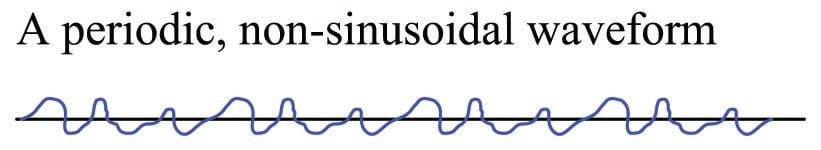
Normal machine vibrations rarely take the form of perfect sinusoidal waves. Although typical vibration waveforms are periodic (i.e. they repeat a pattern over time), they usually do not resemble sine or cosine waves in their shape:
An unfortunate quality of non-sinusoidal waveforms is that they do not lend themselves as readily to mathematical analysis as sinusoidal waves. From the previous discussion on sinusoidal vibrations, we saw how simple it was to take the derivative of a sinusoidal waveform (\({d \over dt} \sin \omega t = \omega \cos \omega t\)), and how well this worked to predict velocity and acceleration from a function describing displacement. Most non-sinusoidal waveforms cannot be expressed as simply and neatly as \(\sin \omega t\), however, and as such are not as easy to mathematically analyze.
Fortunately, though, there is a way to represent non-sinusoidal waveforms as combinations of sinusoidal waveforms. The French mathematician and physicist Jean Baptiste Joseph Fourier (1768-1830) proved mathematically that any periodic waveform, no matter how strange or asymmetrical its shape may be, may be replicated by a specific sum of sine and cosine waveforms of integer-multiple frequencies. That is, any periodic waveform (a periodic function of time, \(f(\omega t)\) being the standard mathematical expression) is equivalent to a series of the following form:
\[f(\omega t) = A_1 \cos \omega t + B_1 \sin \omega t + A_2 \cos 2 \omega t + B_2 \sin 2 \omega t + \cdots A_n \cos n \omega t + B_n \sin n \omega t\]
Here, \(\omega\) represents the fundamental frequency of the waveform, while multiples of \(\omega\) (e.g. \(2 \omega\), \(3 \omega\), \(4 \omega\), etc.) represent harmonic or overtone frequencies of that fundamental. The \(A\) and \(B\) coefficients describe the amplitudes (heights) of each sinusoid. We may break down a typical Fourier series in table form, labeling each term according to frequency:
| Terms | Harmonic | Overtone |
|---|---|---|
| \(A_1 \cos \omega t + B_1 \sin \omega t\) | 1\(^{st}\) harmonic | Fundamental |
| \(A_2 \cos 2 \omega t + B_2 \sin 2 \omega t\) | 2\(^{nd}\) harmonic | 1\(^{st}\) overtone |
| \(A_3 \cos 3 \omega t + B_3 \sin 3 \omega t\) | 3\(^{rd}\) harmonic | 2\(^{nd}\) overtone |
| \(A_4 \cos 4 \omega t + B_4 \sin 4 \omega t\) | 4\(^{th}\) harmonic | 3\(^{rd}\) overtone |
| \(A_n \cos n \omega t + B_n \sin n \omega t\) | \(n^{th}\) harmonic | \((n-1)^{th}\) overtone |
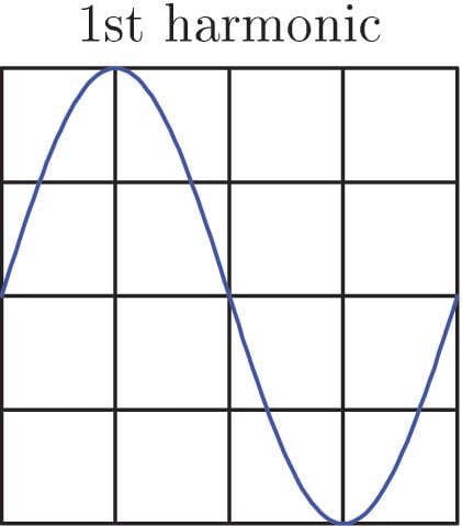
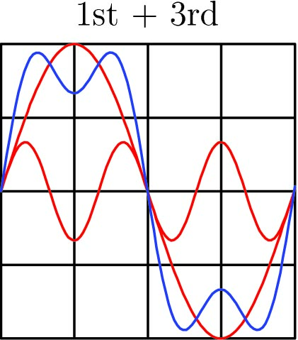
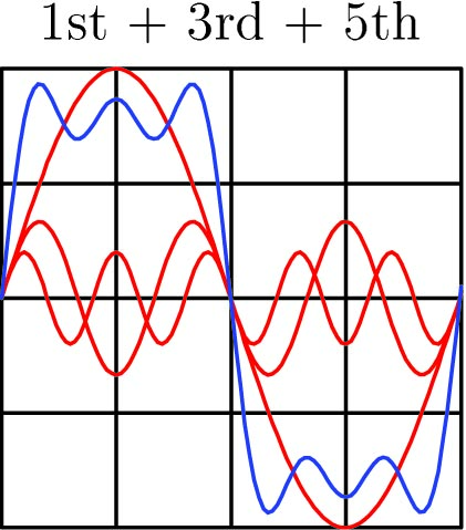
One of the most visually convincing examples of Fourier’s theorem is the ability to describe a square wave as a series of sine waves. Intuition would suggest it is impossible to synthesize a sharp-edged waveform such as a square wave using nothing but rounded sinusoids, but it is indeed possible if one combines an infinite series of sinusoids of successively higher harmonic frequencies, given just the right combination of harmonic frequencies and amplitudes.
The Fourier series for a square wave is as follows:
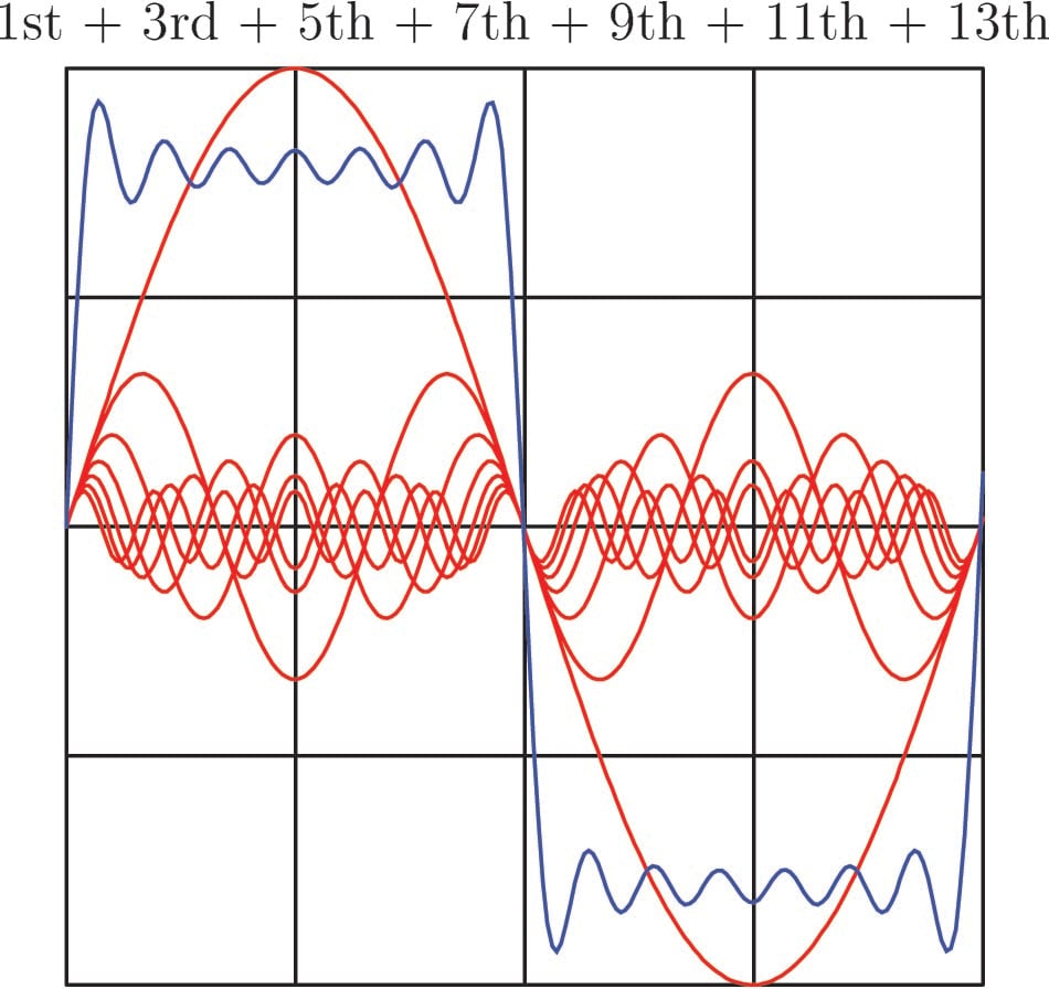
\[\hbox{Square wave} = 1 \sin \omega t + {1 \over 3} \sin 3 \omega t + {1 \over 5} \sin 5 \omega t + {1 \over 7} \sin 7 \omega t + \cdots\]
Such a series would be impossible to numerically calculate, but we may approximate it by adding several of the first (largest) harmonics together to see the resulting shape. In each of the following plots, we see the individual harmonic waveforms plotted in red, with the sum plotted in blue:
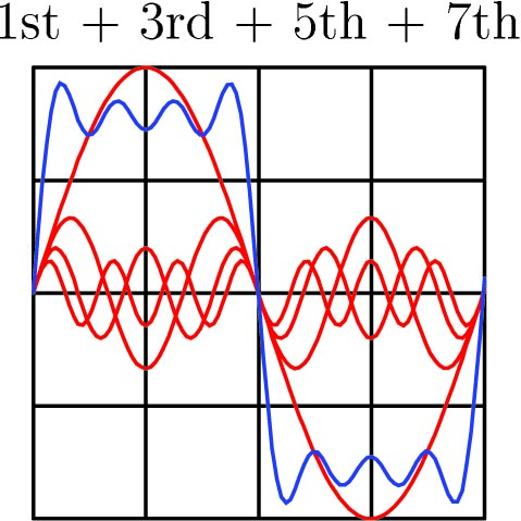
If we continue this pattern up to the 13th harmonic (following the same pattern of diminishing reciprocal amplitudes shown in the Fourier series for a square wave), we see the resultant sum looking more like a square wave:
Continuing on to the 35th harmonic, the resultant sum looks like a square wave with ripples at each rising and falling edge:
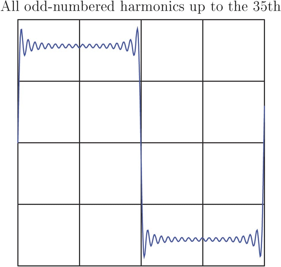
If we were to continue adding successive terms in this infinite series, the resulting superposition of sinusoids would look more and more like a perfect square wave.
The only real question in any practical application is, “What are the \(A\), \(B\), and \(\omega\) coefficient values necessary to describe a particular non-periodic waveform using a Fourier series?” Fourier’s theorem tells us we should be able to represent any periodic waveform – no matter what its shape – by summing together a particular series of sinusoids of just the right amplitudes and frequencies, but actually determining those amplitudes and frequencies is a another matter entirely. Fortunately, modern computational techniques such as the Fast Fourier Transform (or FFT) algorithm make it very easy to sample any periodic waveform and have a digital computer calculate the relative amplitudes and frequencies of its constituent harmonics. The result of a FFT analysis is a summary of the amplitudes, frequencies, and (in some cases) the phase angle of each harmonic.
To illustrate the relationship between a waveform plotted with respect to time versus a Fourier analysis showing component frequencies, I will show a pair of Fourier spectrum plots for two waveforms – one a perfect sinusoid and the other a non-sinusoidal waveform. First, the perfect sinusoid:
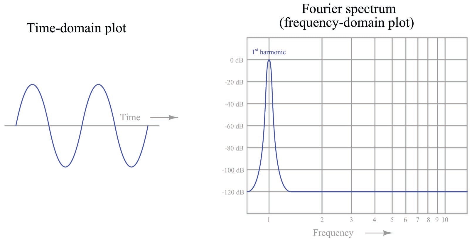
Fourier spectra are often referred to as frequency-domain plots because the x-axis (the “domain” in mathematical lingo) is frequency. A standard oscilloscope-type plot is called a time-domain plot because the x-axis is time. In this first set of plots, we see a perfect sine wave reduced to a single peak on the Fourier spectrum, showing a signal with only one frequency (the fundamental, or 1st harmonic). Here, the Fourier spectrum is very plain because there is only one frequency to display. In other words, the Fourier series for this perfect sinusoid would be:
\[f(\omega t) = 0 \cos \omega t + 1 \sin \omega t + 0 \cos 2 \omega t + 0 \sin 2 \omega t + \cdots 0 \cos n \omega t + 0 \sin n \omega t\]
Only the \(B_1\) coefficient has a non-zero value. All other coefficients are zero because it only takes one sinusoid to perfectly represent this waveform.
Next, we will examine the Fourier analysis of a non-sinusoidal waveform:
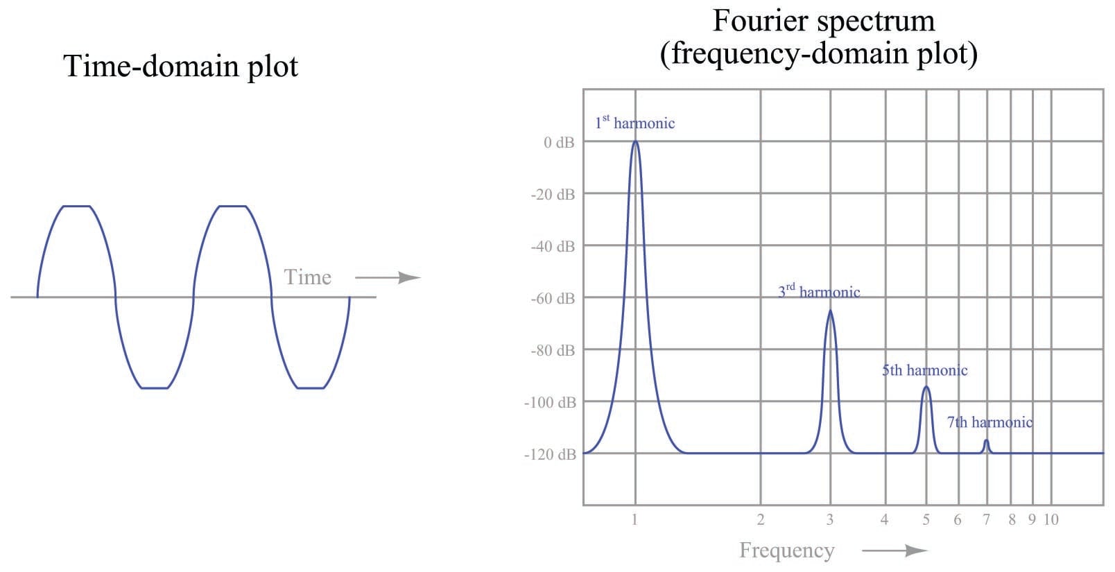
In this second set of plots, we see the waveform is similar to a sine wave, except that it appears “clipped” at the peaks. This waveform is obviously not a perfect sinusoid, and therefore cannot be described by just one of the terms (\(\sin \omega t\)) in a Fourier series. It can, however, be described as equivalent to a series of perfect sinusoids summed together. In this case, the Fourier spectrum shows one sinusoid at the fundamental frequency, plus another (smaller) sinusoid at three times the fundamental frequency (\(3 \omega\)), plus another (yet smaller) sinusoid at the 5th harmonic and another (smaller still!) at the 7th: a series of odd-numbered harmonics.
If each of these harmonics is in phase with each other, we could write the Fourier series as a set of sine terms:
\[f(\omega t) = (0 \hbox{ dB}) \sin \omega t + (-65 \hbox{ dB}) \sin 3 \omega t + (-95 \hbox{ dB}) \sin 5 \omega t + (-115 \hbox{ dB}) \sin 7 \omega t\]
Translating the decibel amplitude values into simple coefficients, we can see just how small these harmonic sinusoids are in comparison to the fundamental:
\[f(\omega t) = 1 \sin \omega t + 0.000562 \sin 3 \omega t + 0.0000178 \sin 5 \omega t + 0.00000178 \sin 7 \omega t\]
If the waveform deviated even further from a perfect sinusoid, we would see a Fourier spectrum with taller harmonic peaks, and perhaps more of them (possibly including some even-numbered harmonics, not just odd-numbered), representing a harmonically “richer” spectrum.
Within the technical discipline of machine vibration analysis, harmonic vibrations are often referred to by labels such as 1X, 2X, and 3X, the integer number corresponding to the harmonic order of the vibration. The fundamental, or first harmonic, frequency of vibration would be represented by “1X” while “2X” and “3X” represent the second- and third-order harmonic frequencies, respectively.
On a practical note, the Fourier analysis of a machine’s vibration waveform holds clues to the successful balancing of that machine. A first-harmonic vibration may be countered by placing an off-center mass on the rotating element 180 degrees out of phase with the offending sinusoid. Given the proper phase (180\(^{o}\) – exactly opposed) and magnitude, any harmonic may be counterbalanced by an off-center mass rotating at the same frequency. In other words, we may cancel any particular harmonic vibration with an equal and opposite harmonic vibration.
If you examine the “crankshaft” of a piston engine, for example, you will notice counterweights with blind holes drilled in specific locations for balancing. These precisely-trimmed counterweights compensate for first-harmonic (fundamental) frequency vibrations resulting from the up-and-down oscillations of the pistons within the cylinders. However, in some engine designs such as inline 4-cylinder arrangements, there are significant harmonic vibrations of a greater order than the fundamental, which cannot be counterbalanced by any amount of weight, in any location, on the rotating crankshaft. The reciprocating motion of the pistons and connecting rods produce periodic vibrations that are non-sinusoidal, and these vibrations (like all periodic, non-sinusoidal waveforms) are equivalent to a series of harmonically-related sinusoidal vibrations.
Any weight attached to the crankshaft will produce a first-order (fundamental) sinusoidal vibration, and that is all. In order to counteract harmonic vibrations of the higher order, the engine requires counterbalance shafts spinning at speeds corresponding to those higher orders. This is why many high-performance inline 4-cylinder engines employ counterbalance shafts spinning at twice the crankshaft speed: to counteract the second-harmonic vibrations created by the reciprocating parts. If an engine designer were so inclined, he or she could include several counterbalance shafts, each one spinning at a different multiple of the crankshaft speed, to counteract as many harmonics as possible. At some point, however, the inclusion of all these shafts and the gearing necessary to ensure their precise speeds and phase shifts would interfere with the more basic design features of the engine, which is why you do not typically see an engine with multiple counterbalance shafts.
The harmonic content of a machine’s vibration signal in and of itself tells us little about the health or balance of that machine. It may be perfectly normal for a machine to have a very “rich” harmonic signature due to convoluted motions of its parts. However, Fourier analysis provides a simple way to quantify complex vibrations and to archive them for future reference. For example, we might gather vibration data on a new machine immediately after installation (including its Fourier spectra on all vibration measurement points) and save this data for safe keeping in the maintenance archives. Later, if and when we suspect a vibration-related problem with this machine, we may gather new vibration data and compare it against the original “signature” spectra to see if anything substantial has changed. Changes in harmonic amplitudes and/or the appearance of new harmonics may point to specific problems inside the machine. Expert knowledge is usually required to interpret the spectral changes and discern what that specific problem (s) might be, but at least this technique does have diagnostic value in the right hands.
