 Facebook
 Google
 GitHub
 Linkedin
Practical Measures of Reliability
In reliability engineering, it is important to be able to quantity the reliability (or conversely, the probability of failure) for common components, and for systems comprised of those components. As such, special terms and mathematical models have been developed to describe probability as it applies to component and system reliability.
Failure rate and MTBF
Perhaps the first and most fundamental measure of (un)reliability is the failure rate of a component or system of components, symbolized by the Greek letter lambda (\(\lambda\)). The definition of “failure rate” for a group of components undergoing reliability tests is the instantaneous rate of failures per number of surviving components:
\[\lambda = {{dN_f \over dt} \over N_s} \hspace{25pt} or \hspace{25pt} \lambda = {{dN_f \over dt} {1 \over N_s}}\]
Where,
\(\lambda\) = Failure rate
\(N_f\) = Number of components failed during testing period
\(N_s\) = Number of components surviving during testing period
\(t\) = Time
The unit of measurement for failure rate (\(\lambda\)) is inverted time units (e.g. “per hour” or “per year”). An alternative expression for failure rate sometimes seen in reliability literature is the acronym FIT (“Failures In Time”), in units of \(10^{-9}\) failures per hour. Using a unit with a built-in multiplier such as \(10^{-9}\) makes it easier for human beings to manage the very small \(\lambda\) values normally associated with high-reliability industrial components and systems.
Failure rate may also be applied to discrete-switching (on/off) components and systems of discrete-switching components on the basis of the number of on/off cycles rather than clock time. In such cases, we define failure rate in terms of cycles (\(c\)) instead of in terms of minutes, hours, or any other measure of time (\(t\)):
\[\lambda = {{dN_f \over dc} \over N_s} \hspace{25pt} or \hspace{25pt} \lambda = {{dN_f \over dc} {1 \over N_s}}\]
One of the conceptual difficulties inherent to the definition of lambda (\(\lambda\)) is that it is fundamentally a rate of failure over time. This is why the calculus notation \(dN_f \over dt\) is used to define lambda: a “derivative” in calculus always expresses a rate of change. However, a failure rate is not the same thing as the number of devices failed in a test, nor is it the same thing as the probability of failure for one or more of those devices. Failure rate (\(\lambda\)) has more in common with the time constant of an resistor-capacitor circuit (\(\tau\)) than anything else.
An illustrative example is helpful here: if we were to test a large batch of identical components for proper operation over some extended period of time with no maintenance or other intervention, the number of failed components in that batch would gradually accumulate while the number of surviving components in the batch would gradually decline. The reason for this is obvious: every component that fails remains failed (with no repair), leaving one fewer surviving component to function. If we limit the duration of this test to a time-span much shorter than the expected lifetime of the components, any failures that occur during the test must be due to random causes (“Acts of God”) rather than component wear-out.
This scenario is analogous to another random process: rolling a large set of dice, counting any “1” roll as a “fail” and any other rolled number as a “survive.” Imagine rolling the whole batch of dice at once, setting aside any dice landing on “1” aside (counting them as “failed” components in the batch), then only rolling the remaining dice the next time. If we maintain this protocol – setting aside “failed” dice after each roll and only continuing to roll “surviving” dice the next time – we will find ourselves rolling fewer and fewer “surviving” dice in each successive roll of the batch. Even though each of the six-sided die has a fixed failure probability of \(1 \over 6\), the population of “failed” dice keeps growing over time while the population of “surviving” dice keeps dwindling over time.
Not only does the number of surviving components in such a test dwindle over time, but that number dwindles at an ever-decreasing rate. Likewise with the number of failures: the number of components failing (dice coming up “1”) is greatest at first, but then tapers off after the population of surviving components gets smaller and smaller. Plotted over time, the graph looks something like this:
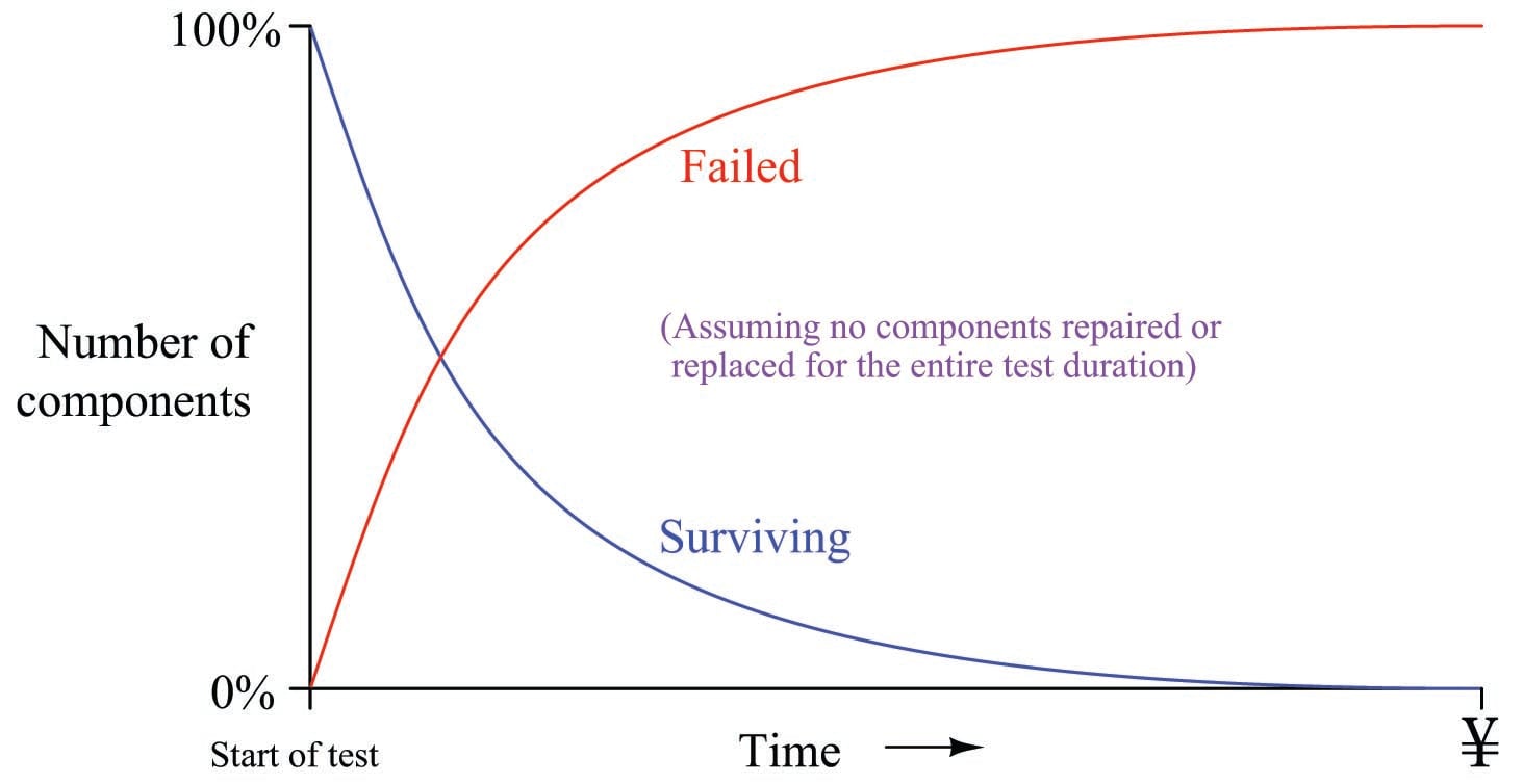
Rapid changes in the failed and surviving component populations occurs at the start of the test when there is the greatest number of functioning components “in play.” As components fail due to random events, the smaller and smaller number of surviving components results in a slower approach for both curves, simply because there are fewer surviving components remaining to fail.
These curves are precisely identical to those seen in RC (resistor-capacitor) charging circuits, with voltage and current tracing complementary paths: one climbing to 100% and the other falling to 0%, but both of them doing so at ever-decreasing rates. Despite the asymptotic approach of both curves, however, we can describe their approaches in an RC circuit with a constant value \(\tau\), otherwise known as the time constant for the RC circuit. Failure rate (\(\lambda\)) plays a similar role in describing the failed/surviving curves of a batch of tested components:
\[N_{surviving} = N_o e^{-\lambda t} \hskip 30pt N_{failed} = N_o \left(1 - e^{-\lambda t}\right)\]
Where,
\(N_{surviving}\) = Number of components surviving at time \(t\)
\(N_{failed}\) = Number of components failed at time \(t\)
\(N_o\) = Total number of components in test batch
\(e\) = Euler’s constant (\(\approx 2.71828\))
\(\lambda\) = Failure rate (assumed to be a constant during the useful life period)
Following these formulae, we see that 63.2% of the components will fail (36.8% will survive) when \(\lambda t\) = 1 (i.e. after one “time constant” has elapsed).
Unfortunately, this definition for lambda doesn’t make much intuitive sense. There is a way, however, to model failure rate in a way that not only makes more immediate sense, but is also more realistic to industrial applications. Imagine a different testing protocol where we maintain a constant sample quantity of components over the entire testing period by immediately replacing each failed device with a working substitute as soon as it fails. Now, the number of functioning devices under test will remain constant rather than declining as components fail. Imagine counting the number of “fails” (dice falling on a “1”) for each batch roll, and then rolling all the dice in each successive trial rather than setting aside the “failed” dice and only rolling those remaining. If we did this, we would expect a constant fraction \(\left(1 \over 6\right)\) of the six-sided dice to “fail” with each and every roll. The number of failures per roll divided by the total number of dice would be the failure rate (lambda, \(\lambda\)) for these dice. We do not see a curve over time because we do not let the failed components remain failed, and thus we see a constant number of failures with each period of time (with each group-roll).
We may mathematically express this using a different formula:
\[\lambda = {{N_f \over t} \over N_o} \hspace{25pt} or \hspace{25pt} \lambda = {{N_f \over t} {1 \over N_o}}\]
Where,
\(\lambda\) = Failure rate
\(N_f\) = Number of components failed during testing period
\(N_o\) = Number of components under test (maintained constant) during testing period by immediate replacement of failed components
\(t\) = Time
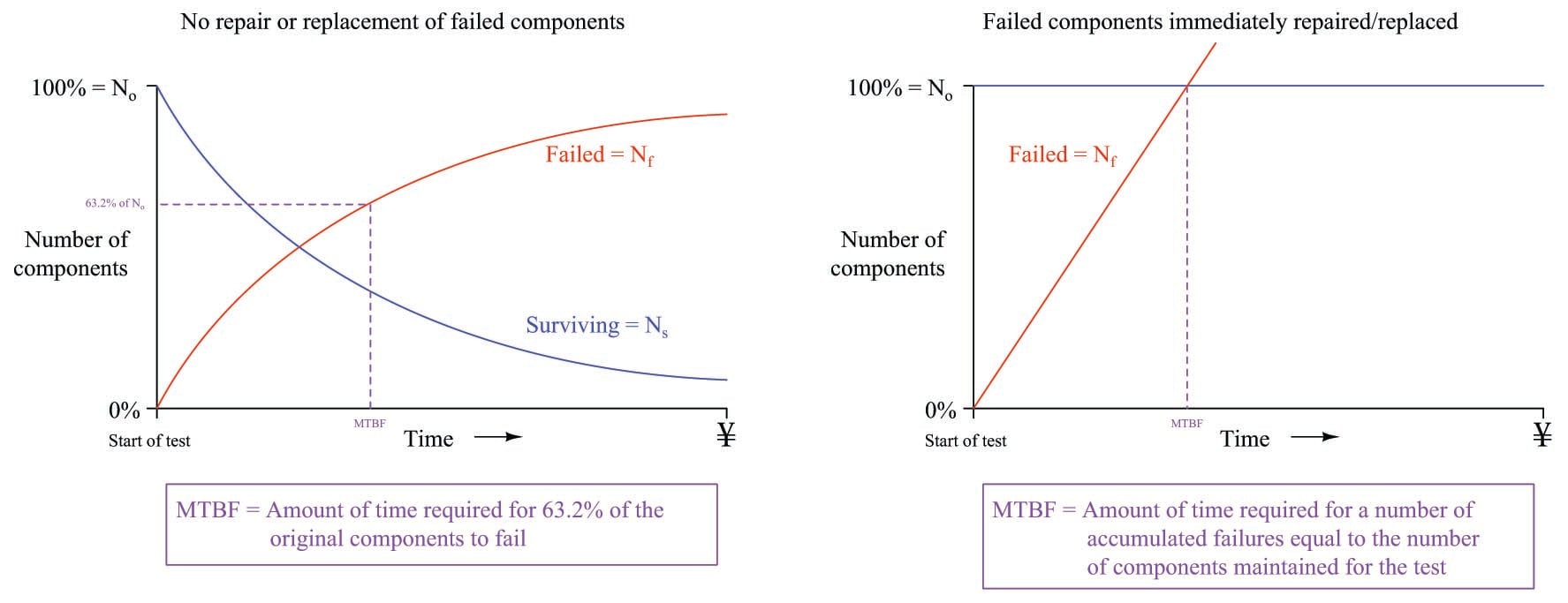
An alternative way of expressing the failure rate for a component or system is the reciprocal of lambda (\(1 \over \lambda\)), otherwise known as Mean Time Between Failures (MTBF). If the component or system in question is repairable, the expression Mean Time To Failure (MTTF) is often used instead. Whereas failure rate (\(\lambda\)) is measured in reciprocal units of time (e.g. “per hour” or “per year”), MTBF is simply expressed in units of time (e.g. “hours” or “years”).
For non-maintained tests where the number of failed components accumulates over time (and the number of survivors dwindles), MTBF is precisely equivalent to “time constant” in an RC circuit: MTBF is the amount of time it will take for 63.2% of the components to fail due to random causes, leaving 36.8% of the component surviving. For maintained tests where the number of functioning components remains constant due to swift repairs or replacement of failed components, MTBF (or MTTF) is the amount of time it will take for the total number of tested components to fail.
It should be noted that these definitions for lambda and MTBF are idealized, and do not necessarily represent all the complexity we see in real-life applications. The task of calculating lambda or MTBF for any real component sample can be quite complex, involving statistical techniques well beyond the scope of instrument technician work.
Simple calculation example: transistor failure rate
Problem: Suppose a semiconductor manufacturer creates a microprocessor “chip” containing 2500000 transistors, each of which is virtually identical to the next in terms of ruggedness and exposure to degrading factors such as heat. The architecture of this microprocessor is such that there is enough redundancy to allow continued operation despite the failure of some of its transistors. This integrated circuit is continuously tested for a period of 1000 days (24000 hours), after which the circuit is examined to count the number of failed transistors. This testing period is well within the useful life of the microprocessor chip, so we know none of the failures will be due to wear-out, but rather to random causes.
Supposing several tests are run on identical chips, with an average of 3.4 transistors failing per 1000-day test. Calculate the failure rate (\(\lambda\)) and the MTBF for these transistors.
Solution: The testing scenario is one where failed components are not replaced, which means both the number of failed transistors and the number of surviving transistors changes over time like voltage and current in an RC charging circuit. Thus, we must calculate lambda by solving for it in the exponential formula.
Using the appropriate formula, relating number of failed components to the total number of components:
\[N_{failed} = N_o \left(1 - e^{-\lambda t}\right)\]
\[3.4 = 2500000 \left(1 - e^{-24000 \lambda}\right)\]
\[1.36 \times 10^{-6} = 1 - e^{-24000 \lambda}\]
\[e^{-24000 \lambda} = 1 - 1.36 \times 10^{-6}\]
\[-24000 \lambda = \ln (1 - 1.36 \times 10^{-6})\]
\[-24000 \lambda = -1.360000925 \times 10^{-6}\]
\[\lambda = 5.66667 \times 10^{-11} \hbox{ per hour} = 0.0566667 \hbox{ FIT}\]
Failure rate may be expressed in units of “per hour,” “Failures In Time” (FIT, which means failures per \(10^{9}\) hours), or “per year” (pa).
\[\hbox{MTBF} = {1 \over \lambda} = 1.7647 \times 10^{10} \hbox{ hours} = 2.0145 \times 10^6 \hbox{ years}\]
Recall that Mean Time Between Failures (MTBF) is essentially the “time constant” for this decaying collection of transistors inside each microprocessor chip.
Simple calculation example: control valve failure rate
Problem: Suppose a control valve manufacturer produces a large number of valves, which are then sold to customers and used in comparable process applications. After a period of 5 years, data is collected on the number of failures these valves experienced. Five years is well within the useful life of these control valves, so we know none of the failures will be due to wear-out, but rather to random causes.
Supposing customers report an average of 15 failures for every 200 control valves in service over the 5-year period, calculate the failure rate (\(\lambda\)) and the MTTF for these control valves.
Solution: The testing scenario is one where failures are repaired in a short amount of time, since these are working valves being maintained in a real process environment. Thus, we may calculate lambda as a simple fraction of failed components to total components.
Using the appropriate formula, relating number of failed components to the total number of components:
\[\lambda = {{N_f \over t} {1 \over N_o}}\]
\[\lambda = {{15 \over 5 \hbox{ yr}} {1 \over 200}}\]
\[\lambda = {3 \over 200 \hbox{ yr}}\]
\[\lambda = 0.015 \hbox{ per year (pa)} = 1.7123 \times 10^{-6} \hbox{ per hour}\]
With this value for lambda being so much larger than the microprocessor’s transistors, it is not necessary to use a unit such as FIT to conveniently represent it.
\[\hbox{MTTF} = {1 \over \lambda} = 66.667 \hbox{ years} = 584000 \hbox{ hours}\]
Recall that Mean Time To Failure (MTTF) is the amount of time it would take to log a number of failures equal to the total number of valves in service, given the observed rate of failure due to random causes. Note that MTTF is largely synonymous with MTBF. The only technical difference between MTBF and MTTF is that MTTF more specifically relates to situations where components are repairable, which is the scenario we have here with well-maintained control valves.
The “bathtub” curve
Failure rate tends to be constant during a component’s useful lifespan where the major cause of failure is random events (“Acts of God”). However, lambda does not remain constant over the entire life of the component or system. A common graphical expression of failure rate is the so-called bathtub curve showing the typical failure rate profile over time from initial manufacture (brand-new) to wear-out:
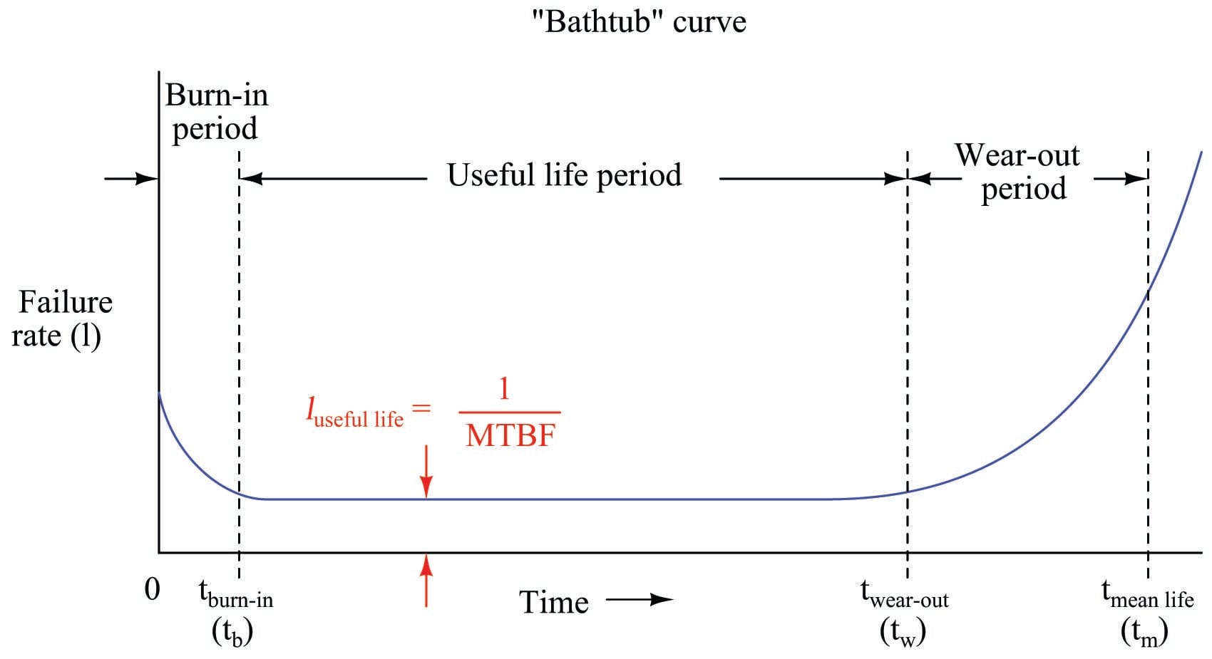
This curve profiles the failure rate of a large sample of components (or a large sample of systems) as they age. Failure rate begins at a relatively high value starting at time zero due to defects in manufacture. Failure rate drops off rapidly during a period of time called the burn-in period where defective components experience an early death. After the burn-in period, failure rate remains relatively constant over the useful life of the components, and this is where we typically define and apply the failure rate (\(\lambda\)). Any failures occurring during this “useful life” period are due to random mishaps (“Acts of God”). Toward the end of the components’ working lives when the components enter the wear-out period, failure rate begins to rise until all components eventually fail. The mean (average) life of a component (\(t_m\)) is the time required for one-half of the components surviving up until the wear-out time (\(t_w\)) to fail, the other half failing after the mean life time.
Several important features are evident in this “bathtub” curve. First, component reliability is greatest between the times of burn-in and wear-out. For this reason, many manufacturers of high-reliability components and systems perform their own burn-in testing prior to sale, so that the customers are purchasing products that have already passed the burn-in phase of their lives. To express this using colloquial terms, we may think of “burnt-in” components as those having already passed through their “growing pains,” and are now “mature” enough to face demanding applications.
Another important measure of reliability is the mean life. This is an expression of a component’s (or system’s) operating lifespan. At first this may sound synonymous with MTBF, but it is not. MTBF – and by extension lambda, since MTBF is the reciprocal of failure rate – is an expression of susceptibility to random (“chance”) failures. Both MTBF and \(\lambda_{useful}\) are quite independent of mean life. In practice, values for MTBF often greatly exceed values for mean life.
To cite a practical example, the Rosemount model 3051C differential pressure transmitter has a suggested useful lifetime of 50 years (based on the expected service life of tantalum electrolytic capacitors used in its circuitry), while its demonstrated MTBF is 136 years. The larger value of 136 years is a projection based on the failure rate of large samples of these transmitters when they are all “young,” which is why one should never confuse MTBF for service life. In reality, components within the instrument will begin to suffer accelerated failure rates as they reach their end of useful lifetime, as the instrument approaches the right-hand end of the “bathtub” curve.
When determining the length of time any component should be allowed to function in a high-reliability system, the mean life (or even better, the wear-out time) should be used as a guide, not the MTBF. This is not to suggest the MTBF is a useless figure – far from it. MTBF simply serves a different purpose, and that is to predict the rate of random failures during the useful life span of a large number of components or systems, whereas mean life predicts the service life period where the component’s failure rate remains relatively constant.
Reliability
Reliability (\(R\)) is the probability a component or system will perform as designed. Like all probability figures, reliability ranges in value from 0 to 1, inclusive. Given the tendency of manufactured devices to fail over time, reliability decreases with time. During the useful life of a component or system, reliability is related to failure rate by a simple exponential function:
\[R = e^{-\lambda t}\]
Where,
\(R\) = Reliability as a function of time (sometimes shown as \(R(t)\))
\(e\) = Euler’s constant (\(\approx 2.71828\))
\(\lambda\) = Failure rate (assumed to be a constant during the useful life period)
\(t\) = Time
Knowing that failure rate is the mathematical reciprocal of mean time between failures (MTBF), we may re-write this equation in terms of MTBF as a “time constant” (\(\tau\)) for random failures during the useful life period:
\[R = e^{-t \over MTBF} \hskip 20pt \hbox{or} \hskip 20pt R = e^{-t \over \tau}\]
This inverse-exponential function mathematically explains the scenario described earlier where we tested a large batch of components, counting the number of failed components and the number of surviving components over time. Like the dice experiment where we set aside each “failed” die and then rolled only the remaining “survivors” for the next trial in the test, we end up with a diminishing number of “survivors” as the test proceeds.
The same exponential function for calculating reliability applies to single components as well. Imagine a single component functioning within its useful life period, subject only to random failures. The longer this component is relied upon, the more time it has to succumb to random faults, and therefore the less likely it is to function perfectly over the duration of its test. To illustrate by example, a pressure transmitter installed and used for a period of 1 year has a greater chance of functioning perfectly over that service time than an identical pressure transmitter pressed into service for 5 years, simply because the one operating for 5 years has five times more opportunity to fail. In other words, the reliability of a component over a specified time is a function of time, and not just the failure rate (\(\lambda\)).
Using dice once again to illustrate, it is as if we rolled a single six-sided die over and over, waiting for it to “fail” (roll a “1”). The more times we roll this single die, the more likely it will eventually “fail” (eventually roll a “1”). With each roll, the probability of failure is \(1 \over 6\), and the probability of survival is \(5 \over 6\). Since survival over multiple rolls necessitates surviving the first roll and and next roll and the next roll, all the way to the last surviving roll, the probability function we should apply here is the “AND” (multiplication) of survival probability. Therefore, the survival probability after a single roll is \(5 \over 6\), while the survival probability for two successive rolls is \(\left(5 \over 6\right)^2\), the survival probability for three successive rolls is \(\left(5 \over 6\right)^3\), and so on.
The following table shows the probabilities of “failure” and “survival” for this die with an increasing number of rolls:
| Number of rolls | Probability of failure (1) | Probability of survival (2, 3, 4, 5, 6) |
|---|---|---|
| 1 | 1 / 6 = 0.16667 | 5 / 6 = 0.83333 |
| 2 | 11 / 36 = 0.30556 | 25 / 36 = 0.69444 |
| 3 | 91 / 216 = 0.42129 | 125 / 216 = 0.57870 |
| 4 | 671 / 1296 = 0.51775 | 625 / 1296 = 0.48225 |
| n | 1 - (5 / 6)n | (5 / 6)n |
A practical example of this equation in use would be the reliability calculation for a Rosemount model 1151 analog differential pressure transmitter (with a demonstrated MTBF value of 226 years as published by Rosemount) over a service life of 5 years following burn-in:
\[R = e^{-5 \over 226}\]
\[R = 0.9781 = 97.81 \%\]
Another way to interpret this reliability value is in terms of a large batch of transmitters. If three hundred Rosemount model 1151 transmitters were continuously used for five years following burn-in (assuming no replacement of failed units), we would expect approximately 293 of them to still be working (i.e. 6.564 random-cause failures) during that five-year period:
\[N_{surviving} = N_o e^{-t \over MTBF}\]
\[\hbox{Number of surviving transmitters} = (300) \left(e^{-5 \over 226}\right) = 293.436\]
\[N_{failed} = N_o \left(1 - e^{-t \over MTBF}\right)\]
\[\hbox{Number of failed transmitters} = 300 \left(1 - e^{-5 \over 226}\right) = 6.564\]
It should be noted that the calculation will be linear rather than inverse-exponential if we assume immediate replacement of failed transmitters (maintaining the total number of functioning units at 300). If this is the case, the number of random-cause failures is simply \(1 \over 226\) per year, or 0.02212 per transmitter over a 5-year period. For a collection of 300 (maintained) Rosemount model 1151 transmitters, this would equate to 6.637 failed units over the 5-year testing span:
\[\hbox{Number of failed transmitters} = (300) \left({5 \over 226} \right) = 6.637\]
Probability of failure on demand (PFD)
Reliability, as previously defined, is the probability a component or system will perform as designed. Like all probability values, reliability is expressed a number ranging between 0 and 1, inclusive. A reliability value of zero (0) means the component or system is totally unreliable (i.e. it is guaranteed to fail). Conversely, a reliability value of one (1) means the component or system is completely reliable (i.e. guaranteed to properly function). In the context of dependability (i.e. the probability that a safety component or system will function when called upon to act), the unreliability of that component or system is referred to as PFD, an acronym standing for Probability of Failure on Demand. Like dependability, this is also a probability value ranging from 0 to 1, inclusive. A PFD value of zero (0) means there is no probability of failure (i.e. it is 100% dependable – guaranteed to properly perform when needed), while a PFD value of one (1) means it is completely undependable (i.e. guaranteed to fail when activated). Thus:
\[\hbox{Dependability} + \hbox{PFD} = 1\]
\[\hbox{PFD} = 1 - \hbox{Dependability}\]
\[\hbox{Dependability} = 1 - \hbox{PFD}\]
Obviously, a system designed for high dependability should exhibit a small PFD value (very nearly 0). Just how low the PFD needs to be is a function of how critical the component or system is to the fulfillment of our human needs.
The degree to which a system must be dependable in order to fulfill our modern expectations is often surprisingly high. Suppose someone were to tell you the reliability of seatbelts in a particular automobile was 99.9 percent (0.999). This sounds rather good, doesn’t it? However, when you actually consider the fact that this degree of probability would mean an average of one failed seatbelt for every 1000 collisions, the results are seen to be rather poor (at least to modern American standards of expectation). If the dependability of seatbelts is 0.999, then the PFD is 0.001:
\[\hbox{PFD} = 1 - \hbox{Dependability}\]
\[\hbox{PFD} = 1 - 0.999\]
\[\hbox{PFD} = 0.001\]
Let’s suppose an automobile manufacturer sets a goal of only 1 failed seatbelt in any of its cars during a 1 million unit production run, assuming each and every one of these cars were to crash. Assuming four seatbelts per car, this equates to a \(1 \over 4000000\) PFD. The necessary dependability of this manufacturer’s seatbelts must therefore be:
\[\hbox{Dependability} = 1 - \hbox{PFD} = 1 - {1 \over 4000000} = 0.99999975\]
Thus, the dependability of these seatbelts must be 99.999975% in order to fulfill the goal of only 1 (potential) seatbelt failure out of 4 million seatbelts produced.
A common order-of-magnitude expression of desired reliability is the number of “9” digits in the reliability value. A reliability value of 99.9% would be expressed as “three nine’s” and a reliability value of 99.99% as “four nine’s.” Expressed thusly, the seatbelt dependability must be “six nine’s” in order to achieve the automobile manufacturer’s goal.
