 Facebook
 Google
 GitHub
 Linkedin
Comparison of Op-Amp Circuits With Analogous Pneumatic Mechanisms
Self-balancing pneumatic instrument mechanisms are very similar to negative-feedback operational amplifier circuits, in that negative feedback is used to generate an output signal in precise proportion to an input signal. This section compares simple operational amplifier (“opamp”) circuits with analogous pneumatic mechanisms for the purpose of illustrating how negative feedback works, and learning how to generally analyze pneumatic mechanisms.
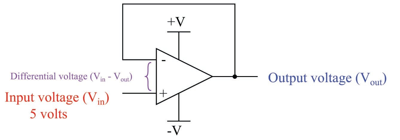
In the following illustration, we see an opamp with no feedback (open loop), next to a baffle/nozzle mechanism with no feedback (open loop):
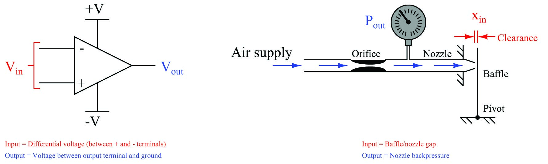
For each system there is an input and an output. For the opamp, input and output are both electrical (voltage) signals: \(V_{in}\) is the differential voltage between the two input terminals, and \(V_{out}\) is the single-ended voltage measured between the output terminal and ground. For the baffle/nozzle, the input is the physical gap between the baffle and nozzle (\(x_{in}\)) while the output is the backpressure indicated by the pressure gauge (\(P_{out}\)).
Both systems have very large gains. Operational amplifier open-loop gains typically exceed 200000 (over 100 dB), and we have already seen how just a few thousandths of an inch of baffle motion is enough to drive the backpressure of a nozzle nearly to its limits (supply pressure and atmospheric pressure, respectively).
Gain (\(A\)) is always defined as the ratio between output and input for a system. Mathematically, it is the quotient of output change and input change, with “change” represented by the triangular Greek capital-letter delta (\(\Delta\)):
\[\hbox{Gain} = A = {\Delta \hbox{Output} \over \Delta \hbox{Input}}\]
Normally, gain is a unitless ratio. We can easily see this for the opamp circuit, since both output and input are voltages, any unit of measurement for voltage would cancel in the quotient, leaving a unitless quantity. This is not so evident in the baffle/nozzle system, with the output represented in units of pressure and the input represented in units of distance.
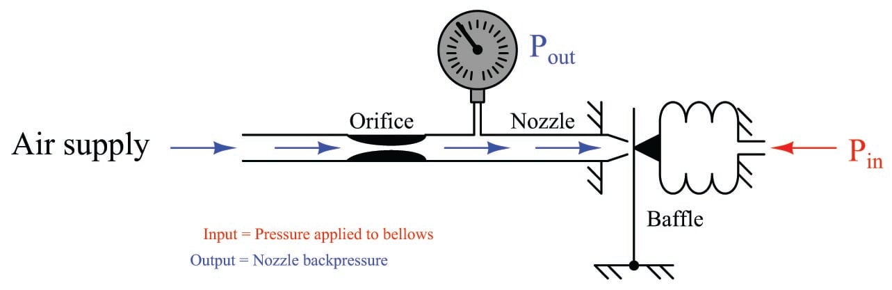
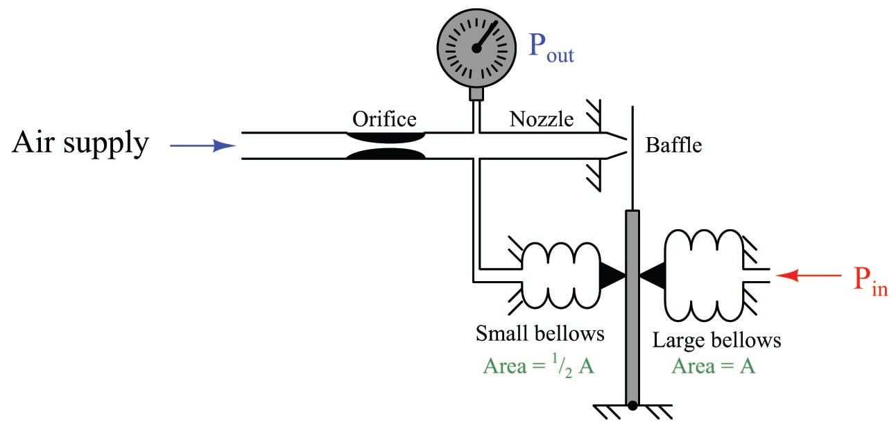
If we were to add a bellows to the baffle/nozzle mechanism, we would have a system that inputs and outputs fluid pressure, allowing us to more formally define the gain of the system as a unitless ratio of \(\Delta P_{out} \over \Delta P_{in}\):
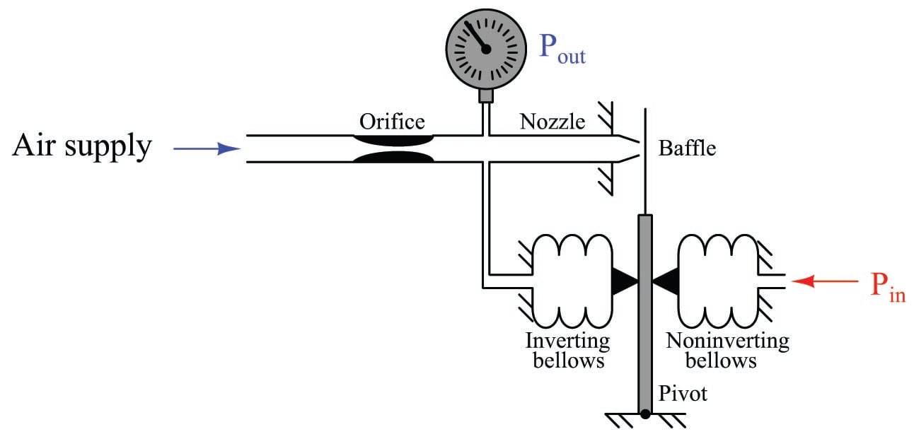
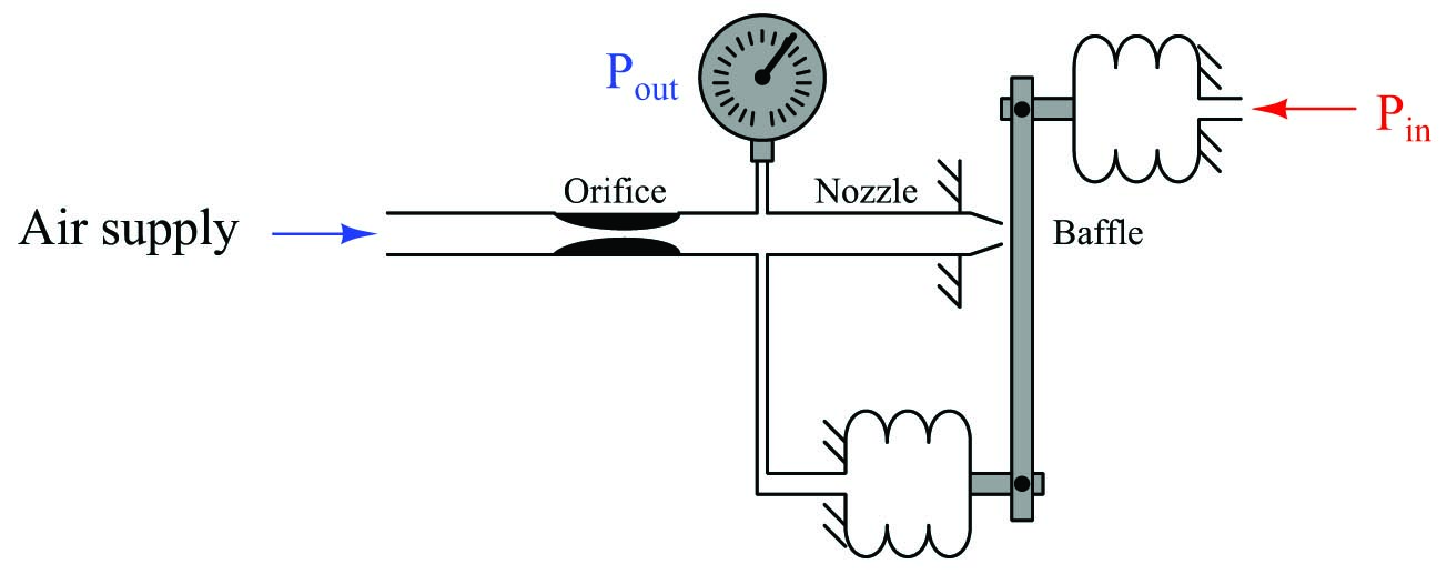
We may modify this mechanism slightly to make it an even more realistic analogue of an operational amplifier circuit by adding a second input bellows in direct opposition to the first:
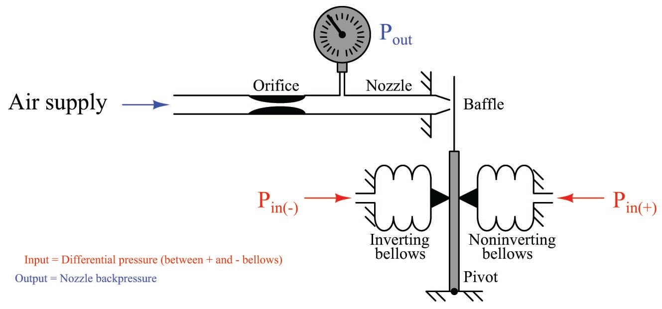
Now our mechanism is a differential-input pneumatic relay. Pressure applied to the “noninverting” input bellows presses the baffle toward the nozzle, causing the output pressure to rise dramatically. Pressure applied to the “inverting” input bellows presses the baffle away from the nozzle, causing the output pressure to fall dramatically. Exactly equal pressures simultaneously applied to both bellows causes no baffle motion at all, resulting in no change in output pressure. This is analogous to an electronic operational amplifier: positive voltage applied to the noninverting (+) input strongly drives the output voltage more positive, while positive voltage applied to the inverting (\(-\)) input strongly drives the output voltage more negative.
Given the extreme sensitivity of a baffle/nozzle mechanism, the pneumatic gain of this device will be quite large. Like its electronic counterpart – the opamp circuit – miniscule input signal levels are sufficient to fully saturate the output.
Electronic operational amplifiers and pneumatic relays find their greatest application where we use feedback, sending all or part of the output signal back to one of the inputs of the device. The most common form of feedback is negative feedback, where the output signal works in such a way as to negate (compensate) itself. The general effect of negative feedback is to decrease the gain of a system, and also make that system’s response more linear over the operating range. This is not an easy concept to grasp, however, and so we will explore the effect of adding negative feedback in detail for both systems.
The simplest implementation of negative feedback is a condition where the entire strength of the output signal gets “fed back” to the amplifier system in degenerative fashion. For an opamp, this simply means connecting the output terminal directly to the inverting input terminal, to form a circuit known as a voltage follower:
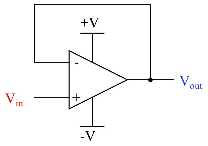
We call this “negative” or “degenerative” feedback because its effect is counteractive in nature. If the output voltage rises too high, the effect of feeding this signal to the inverting input will be to bring the output voltage back down again. Likewise, if the output voltage is too low, the inverting input will sense this and act to bring it back up again. Self-correction is the hallmark of any negative-feedback system.
Having connected the inverting input directly to the output of the opamp leaves us with the noninverting terminal as the sole input. Thus, our input voltage signal is a ground-referenced voltage just like the output. Electronics students learn that the voltage gain of this circuit is unity (1), meaning that the output will assume whatever voltage level is present at the input, within the limits of the opamp’s power supply. This is why the circuit is called a “voltage follower”: the output voltage mimics, or follows, the input voltage. If we were to send a voltage signal of 5 volts to the noninverting terminal of this opamp circuit, it would output 5 volts, provided that the power supply exceeds 5 volts in potential from ground. What is not always taught to electronics students is why this is true.
Let’s mathematically analyze why the gain of a “voltage follower” opamp circuit is unity. First, we will start with the equation representing the open-loop output of an opamp, as a function of its differential input voltage:
\[V_{out} = A_{OL}(V_{in(+)} - V_{in(-)})\]
As stated before, the open-loop voltage gain of an opamp is typically very large (\(A_{OL}\) = 200000 or more!) which means only a tiny voltage difference between the noninverting and inverting inputs \((V_{in(+)} - V_{in(-)})\) is necessary to drive the opamp’s output voltage to saturation.
Connecting the opamp’s output terminal to its own inverting input terminal simplifies the scenario because it makes those two terminals equipotential to each other (i.e. the output and inverting input terminals now have the same potential at all times):
With these two terminals directly connected, \(V_{out}\) and \(V_{in(-)}\) are now one and the same. This means we may substitute \(V_{out}\) for \(V_{in(-)}\) in the equation, while \(V_{in(+)}\) simply becomes \(V_{in}\) since it is now the only remaining input. Reducing the equation to the two variables of \(V_{out}\) and \(V_{in}\) and a constant (\(A_{OL}\)) allows us to solve for overall voltage gain (\(V_{out} \over V_{in}\)) as a function of the opamp’s internal voltage gain (\(A_{OL}\)). The following sequence of algebraic manipulations shows how this is done:
\[V_{out} = A_{OL}(V_{in} - V_{out})\]
\[V_{out} = A_{OL}V_{in} - A_{OL}V_{out}\]
\[A_{OL}V_{out} + V_{out} = A_{OL}V_{in}\]
\[V_{out} (A_{OL} + 1) = A_{OL}V_{in}\]
\[\hbox{Overall gain} = {V_{out} \over V_{in}} = {A_{OL} \over {A_{OL} + 1}}\]
If we assume an internal opamp gain of 200000, the overall gain will be very nearly equal to unity (0.999995). Moreover, this near-unity gain will remain quite stable despite large changes in the opamp’s internal (open-loop) gain. The following table shows the effect of major \(A_{OL}\) changes on overall voltage gain (\(A_V\)):
Internal gain -- Overall gain
| \(A_{OL}\) | \(A_V\) |
|---|---|
| 100000 | 0.99999 |
| 200000 | 0.999995 |
| 300000 | 0.999997 |
| 500000 | 0.999998 |
| 1000000 | 0.999999 |
Note how an order of magnitude change in \(A_{OL}\) (from 100000 to 1000000) results is a miniscule change in overall voltage gain (from 0.99999 to 0.999999). Negative feedback clearly has a stabilizing effect on the closed-loop gain: the internal gain of the operational amplifier may drift considerably over time with negligible effect on the voltage follower circuit’s overall gain. It was this principle that led Harold Black in the late 1920’s to apply negative feedback to the design of very stable telephone amplifier circuits. His discovery led to the development of electronic amplifiers exhibiting very stable gains despite internal changes such as vacuum tube aging, power supply drift, etc.
If we subject our voltage follower circuit to a constant input voltage of exactly 5 volts, we may expand the table to show the effect of changing open-loop gain on the output voltage, and also the differential voltage appearing between the opamp’s two input terminals:
Internal gain -- Overall gain -- Output voltage -- Differential voltage
| \(A_{OL}\) | \(A_V\) | \(V_{out}\) | \(V_{in(+)} - V_{in(-)}\) |
|---|---|---|---|
| 100000 | 0.99999 | 4.99995 | 0.00005 |
| 200000 | 0.999995 | 4.999975 | 0.000025 |
| 300000 | 0.999997 | 4.99998 | 0.00002 |
| 500000 | 0.999998 | 4.99999 | 0.00001 |
| 1000000 | 0.999999 | 4.999995 | 0.000005 |
With such extremely high open-loop voltage gains, it hardly requires any difference in voltage between the two input terminals to generate the necessary output voltage to match the input. Negative feedback has “tamed” the opamp’s extremely large gain to a value that is nearly 1. Thus, \(V_{out} = V_{in}\) for all practical purposes, and the opamp’s differential voltage input is zero for all practical purposes.
One of the “simplifying assumptions” electronics technicians and engineers make when analyzing opamp circuits is that the differential input voltage in any negative feedback circuit is zero. As we see in the above table, this assumption is very nearly true. Following this assumption to its logical consequence allows us to predict the output voltage of any negative feedback opamp circuit quite simply. For example:
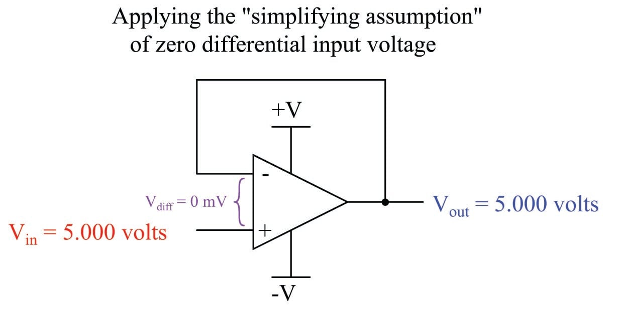
Building on this assumption, we may conclude that the opamp will output whatever voltage it must to maintain zero differential voltage between its inputs. In other words, we assume zero volts between the two input terminals of the opamp, then calculate what the output voltage must be in order for that condition to remain true. If we assume there will be zero differential voltage between the two input terminals of the opamp, we see that the output voltage will exactly equal the input voltage, for that is what must happen here in order for the two opamp input terminals to see equal potentials. We don’t even need to evaluate a mathematical formula to tell what the voltage follower will do with a 5 volt input – the simplifying assumption lets us directly conclude \(V_{out} = V_{in}\).
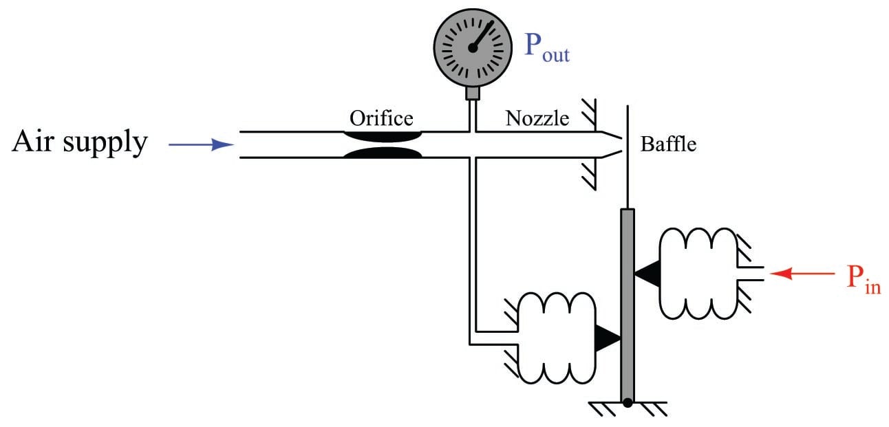
Now let us apply negative feedback to our differential-input pneumatic relay and analyze it similarly. The simplest and most direct form of negative feedback is to connect the output pressure line to the inverting bellows. This leaves only one input pressure port remaining:
It should be clear that the inverting bellows, which now experiences the same pressure (\(P_{out}\)) as the pressure gauge, introduces negative feedback into the system. If the output pressure happens to rise too high, the baffle will be pushed away from the nozzle by the force of the feedback bellows, causing backpressure to decrease and stabilize. Likewise, if the output pressure happens to go too low, the baffle will move closer to the nozzle and cause the backpressure to rise again.
As we have seen already, the baffle/nozzle is exceptionally sensitive: only a few thousandths of an inch of motion being sufficient to saturate the nozzle backpressure to either extreme (supply air pressure or zero, depending on which direction the baffle moves). This is analogous to the high gain of an operational amplifier, requiring only a few microvolts of potential difference between the input terminals to saturate the amplifier’s output to full “rail” voltage. This being the case, we may conclude the nozzle backpressure can assume any value needed with negligible pressure difference between the two opposed bellows. From this we may conclude the system naturally seeks a condition where the pressure inside the feedback bellows matches the pressure inside the “input” bellows. In other words, \(P_{out}\) will (very nearly) equal \(P_{in}\) with negative feedback in effect.
Introducing negative feedback to the opamp led to a condition where the differential input voltage was held to (nearly) zero. In fact, this potential was so small as to safely consider it a constant zero microvolts for the purpose of more easily analyzing the output response of the system. We may make the exact same “simplifying assumption” for the pneumatic mechanism: we will assume zero baffle/nozzle gap motion (i.e. the gap remains constant) so long as negative feedback is at work.
Building on this assumption, we may conclude the nozzle backpressure will rise or fall to whatever value it must in order to maintain a constant baffle/nozzle gap at all times. In other words, we may analyze the operation of a pneumatic feedback mechanism for any given input condition by assuming a constant baffle/nozzle gap, then calculate what the output pressure must be in order for that assumption to remain true.
If we simply assume the baffle/nozzle gap will be held constant through the action of negative feedback, we may conclude in this case that the output pressure is exactly equal to the input pressure, since that is what must happen in order for the two pressures to exactly oppose each other through two identical bellows to hold the baffle at a constant gap from the nozzle.
The analytical technique of assuming perfect balance in a negative feedback system works just as well for more complicated systems. Consider the following opamp circuit:
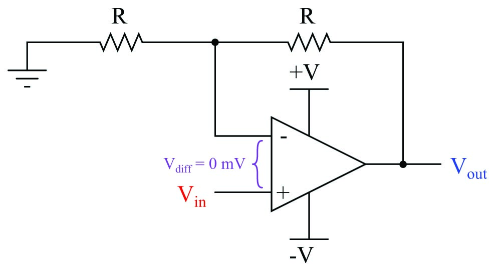
Here, negative feedback occurs through a voltage divider from the output terminal to the inverting input terminal, such that only one-half of the output voltage gets “fed back” degeneratively. If we follow our simplifying assumption that perfect balance (zero difference of voltage) will be achieved between the two opamp input terminals due to the balancing action of negative feedback, we conclude \(V_{out}\) must be exactly twice the magnitude of \(V_{in}\). In other words, the output voltage must increase to twice the value of the input voltage in order for the divided feedback signal to exactly match the input signal. Thus, feeding back half the output voltage yields an overall voltage gain of two.
If we make the same (analogous) change to the pneumatic system, we see the same effect:
Here, the feedback bellows has half the surface area of the input bellows. This results in half the amount of force applied to the beam for the same amount of pressure. If we follow our simplifying assumption that perfect balance (zero baffle motion) will be achieved due to the balancing action of negative feedback, we conclude \(P_{out}\) must be exactly twice the magnitude of \(P_{in}\). In other words, the output pressure must increase to twice the value of the input pressure in order for the divided feedback force to exactly match the input force and prevent the baffle from moving. Thus, our pneumatic mechanism has a pressure gain of two, just like the opamp circuit with divided feedback had a voltage gain of two.
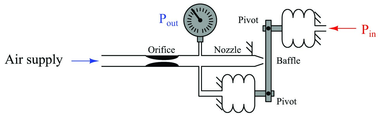
We could have achieved the same effect by moving the feedback bellows to a lower position on the force beam instead of changing its surface area:
This arrangement effectively reduces the feedback force by placing the feedback bellows at a mechanical disadvantage to the input bellows. If the distance between the feedback bellows tip and the force beam pivot is exactly half the distance between the input bellows tip and the force beam pivot, the effective force ratio will be one-half. The result of this “divided” feedback force is that the output pressure must rise to twice the value of the input pressure, since the output pressure is at a mechanical disadvantage to the input. Once again, we see a balancing mechanism with a gain of two.
Pneumatic instruments built such that bellows’ forces directly oppose one another in the same line of action to constrain the motion are known as “force balance” systems. Instruments built such that bellows’ forces oppose one another through different lever lengths pivoting around the same fulcrum point (such as in the last system) are technically known as “moment balance” systems. Instead of two equal forces balancing, we have two equal “moments” or torques balancing. However, one will often find that “moment balance” instruments are commonly referred to as “force balance” because the two principles are so similar. In either case, the result of the balance is that actual motion is constrained to an absolute minimum, like a tug-of-war where the two sides are perfectly matched in pulling force.
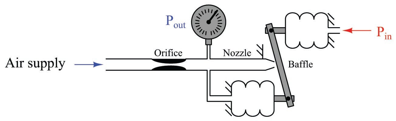
An entirely different classification of pneumatic instrument is known as motion balance. The same “simplifying assumption” of zero baffle/nozzle gap motion holds true for the analysis of these mechanisms as well:
In this particular mechanism there is no fixed pivot for the beam. Instead, the beam hangs between the ends of two bellows units, affixed by pivoting links. As input pressure increases, the input bellows expands outward, attempting to push the beam closer to the nozzle. However, if we follow our assumption that negative feedback holds the nozzle gap constant, we see that the feedback bellows must expand the same amount, and thus (if it has the same area and spring characteristics as the input bellows) the output pressure must equal the input pressure:
We call this a motion balance system instead of a force balance system because we see two motions working in complementary fashion to maintain a constant baffle/nozzle gap instead of two forces working against each other to maintain all components in their original positions.
The distinction between motion-balance and force-balance is a source of confusion for many people, but it is an important concept to master in order to analyze the responses of each and to understand how to calibrate each type of instrument. Perhaps the easiest way to distinguish one from the other is to apply the “simplifying assumption” of a constant baffle/nozzle gap and ask the question, “Must the components move as the signal pressures explore their full ranges?” An analogy to help distinguish force-balance from motion-balance is that of tug-of-war contestants versus ballroom dancers. Two people competing in a tug-of-war maintain a steady gap between themselves and the line only by precisely countering each other’s force: if their forces are perfectly balanced (equal and opposite), they will not move relative to the line. By contrast, two ballroom dancers maintain a steady gap between themselves only by moving the same distance: if their motions are perfectly balanced, the gap between them will not change. Again, the same question applies: do the people actually move in the act of maintaining equilibrium? If so, theirs is a motion-balance system; if not, theirs is a force-balance system.
In a force-balance pneumatic mechanism, the components (ideally) do not move. In fact, if there were such a thing as an infinitely sensitive baffle/nozzle mechanism (where the baffle/nozzle gap held perfectly constant at all times), there would be absolutely no motion at all occurring in a force-balance mechanism! However, even with an infinitely sensitive baffle/nozzle detector, a motion-balance mechanism would still visibly move in its effort to keep the baffle-nozzle gap constant as the pneumatic pressures rose and fell over their respective ranges. This is the most reliable “test” I have found to distinguish one type of mechanism from the other.
The gain of a motion-balance pneumatic instrument may be changed by altering the bellows-to-nozzle distance such that one of the two bellows has more effect than the other. For instance, this system has a gain of 2, since the feedback bellows must move twice as far as the input bellows in order to maintain a constant nozzle gap:
Force-balance (and moment-balance) instruments are generally considered more accurate than motion-balance instruments because motion-balance instruments rely on the pressure elements (bellows, diaphragms, or bourdon tubes) possessing predictable spring characteristics. Since pressure must accurately translate to motion in a motion-balance system, there must be a predictable relationship between pressure and motion in order for the instrument to maintain accuracy. If anything happens to affect this pressure/motion relationship such as metal fatigue or temperature change, the instrument’s calibration will drift. Since there is negligible motion in a force-balance system, pressure element spring characteristics are irrelevant to the operation of these devices, and their calibrations remain more stable over time.
Both force- and motion-balance pneumatic instruments are usually equipped with an amplifying relay between the nozzle backpressure chamber and the feedback bellows. The purpose of an amplifying relay in a self-balancing pneumatic system is twofold: first, it boosts the open-loop gain of the mechanism so that its overall gain may be more predictable and stable; second, it provides additional flow capacity to fill and empty long pneumatic signal tubes necessary to convey the output air pressure signal to remote locations. The following illustration shows how a pneumatic amplifying relay may be used to improve the performance of our demonstration force-balance mechanism:
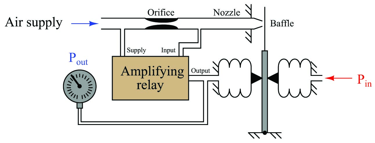
Adding a relay to a self-balancing pneumatic system is analogous to increasing the open-loop voltage gain of an opamp (\(A_{OL}\)) by several-fold: it makes the overall gain closer to ideal. The overall gain of the system, though, is dictated by the ratio of bellows leverage on the force beam, just like the overall gain of a negative-feedback opamp circuit is dictated by the feedback network and not by the opamp’s internal (open-loop) voltage gain.
