 Facebook
 Google
 GitHub
 Linkedin
Introduction to Calculus
Calculus. Few areas of mathematics are as powerfully useful in describing and analyzing the physical world as calculus, the mathematical study of changes. Calculus also happens to be tremendously confusing to most students first encountering it. A great deal of this confusion stems from mathematicians’ insistence on rigor and denial of intuition.
Look around you right now. Do you see any mathematicians? If not, good – you can proceed in safety. If so, find another location to begin reading the rest of this chapter. I will frequently appeal to practical example and intuition in describing the basic principles of single-variable calculus, for the purpose of expanding your mathematical “vocabulary” to be able to describe and better understand phenomena of change related to instrumentation.
Silvanus P. Thompson, in his wonderful book Calculus Made Simple, originally published in 1910, began his text with a short chapter entitled, “To Deliver You From The Preliminary Terrors.” I will follow his lead by similarly introducing you to some of the notations frequently used in calculus, along with very simple (though not mathematically rigorous) definitions.
When we wish to speak of a change in some variable’s value (let’s say \(x\)), it is common to precede the variable with the capital Greek letter “delta” as such:
\[\Delta x = Change~in~x\]
An alternative interpretation of the “delta” symbol (\(\Delta\)) is to think of it as denoting a difference between two values of the same variable. Thus, \(\Delta x\) could be taken to mean “the difference between two values of \(x\)”. The cause of this difference is not important right now: it may be the difference between the value of \(x\) at one point in time versus another point in time, it may be the difference between the value of \(x\) at one point in space versus another point in space, or it may simply be the difference between values of \(x\) as it relates to some other variable (e.g. \(y\)) in a mathematical function. If we have some variable such as \(x\) that is known to change value relative to some other variable (e.g. time, space, \(y\)), it is nice to be able to express that change using precise mathematical symbols, and this is what the “delta” symbol does for us.
For example, if the temperature of a furnace (\(T\)) increases over time, we might wish to describe that change in temperature as \(\Delta T\):
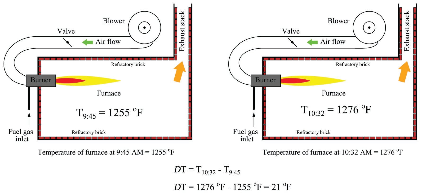
The value of \(\Delta T\) is nothing more than the difference (subtraction) between the recent temperature and the previously recorded temperature. A rising temperature over time thus yields a positive value for \(\Delta T\), while a falling temperature over time yields a negative value for \(\Delta T\).
We could also describe differences between the temperature of two locations (rather than a difference of temperature between two times) by the notation \(\Delta T\), such as this example of heat transfer through a heat-conducting wall where one side of the wall is hotter than the other:
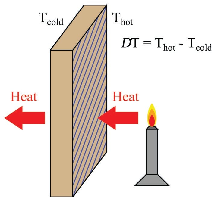
Once again, \(\Delta T\) is calculated by subtracting one temperature from another. Here, the sign (positive or negative) of \(\Delta T\) denotes the direction of heat flow through the thickness of the wall.
One of the major concerns of calculus is changes or differences between variable values lying very close to each other. In the context of a heating furnace, this could mean increases in temperature over minuscule time periods. In the context of heat flowing through a wall, this could mean differences in temperature sampled between points within the wall immediately adjacent each other. If our desire is to express the change in a variable between neighboring points along a continuum rather than over some discrete period, we may use a different notation than the capital Greek letter delta (\(\Delta\)); instead, we use a lower-case Roman letter \(d\) (or in some cases, the lower-case Greek letter delta: \(\delta\)).
Thus, a change in furnace temperature from one instant in time to the next could be expressed as \(dT\) (or \(\delta T\)), and, likewise, a difference in temperature between two adjacent positions within the heat-conducting wall could also be expressed as \(dT\) (or \(\delta T\)). Just as with the “delta” (\(\Delta\)) symbol, the changes references by either \(d\) or \(\delta\) may occur over a variety of different domains.
We even have a unique name for this concept of extremely small differences: whereas \(\Delta T\) is called a difference in temperature, \(dT\) is called a differential of temperature. The concept of a differential may seem redundant to you right now, but they are actually quite powerful for describing continuous changes, especially when one differential is related to another differential by ratio (something we call a derivative).
Another major concern in calculus is how quantities accumulate, especially how differential quantities add up to form a larger whole. A furnace’s temperature rise since start-up (\(\Delta T_{total}\)), for example, could be expressed as the accumulation (sum) of many temperature differences (\(\Delta T\)) measured periodically. The total furnace temperature rise calculated from a sampling of temperature once every minute from 9:45 to 10:32 AM could be written as:
\[\Delta T_{total} = \Delta T_{9:45} + \Delta T_{9:46} + \cdots \Delta T_{10:32} = \hbox{Total temperature rise over time, from 9:45 to 10:32}\]
A more sophisticated expression of this series uses the capital Greek letter sigma (meaning “sum of” in mathematics) with notations specifying which temperature differences to sum:
\[\Delta T_{total} = \sum_{n=9:45}^{10:32} \Delta T_n = \hbox{Total temperature rise over time, from 9:45 to 10:32}\]
However, if our furnace temperature monitor scans at an infinite pace, measuring temperature differentials (\(dT\)) and summing them in rapid succession, we may express the same accumulated temperature rise as an infinite sum of infinitesimal (infinitely small) changes, rather than as a finite sum of temperature changes measured once every minute. Just as we introduced a unique mathematical symbol to represent differentials (\(d\)) over a continuum instead of differences (\(\Delta\)) over discrete periods, we will introduce a unique mathematical symbol to represent the summation of differentials (\(\int\)) instead of the summation of differences (\(\sum\)):
\[\Delta T_{total} = \int_{9:45}^{10:32} dT = \hbox{Total temperature rise over time, from 9:45 to 10:32}\]
This summation of infinitesimal quantities is called integration, and the elongated “S” symbol (\(\int\)) is the integral symbol.
These are the two major ideas and notations of calculus: differentials (tiny changes represented by \(d\) or \(\delta\)) and integrals (accumulations represented by \(\int\)). Now that wasn’t so frightening, was it?
