 Facebook
 Google
 GitHub
 Linkedin
Mathematical Problem-solving Techniques
Some problem-solving techniques are unique to quantitative problems, involving mathematical calculations. In this section we will explore some useful tips to help you solve such problems.
Manipulating algebraic equations
One of the most useful problem-solving techniques in all of algebra is the art of manipulating, or re-writing, equations to solve for a particular variable. The key to this technique is the fact that we may subject an equation to any mathematical operation we desire, so long as we apply that same operation to both sides of the equation.
Let us begin with an illustration showing why this is true. We will represent the equation \(x + 9 = y\) as a balance-beam scale, showing the quantity \(x + 9\) in one pan of the scale and \(y\) in the other pan:
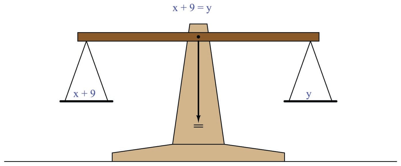
The balance-beam analogy merely represents the fact that the two expressions \(x + 9\) and \(y\) are equal; that is to say, they possess the same mathematical value as described by the equation \(x + 9 = y\). It should be intuitively obvious that this equality will remain unaltered if we were to add some equal quantity to both sides of the equation, such as the number 3:
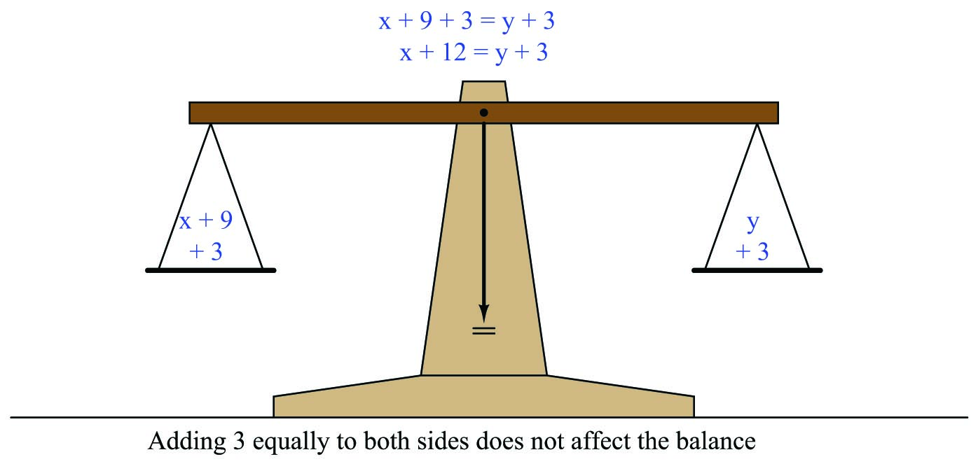
If the left-hand quantity is now larger by 3 units, and the right-hand quantity is also larger by 3 units, and those two quantities began as equal to each other, than those two quantities must still remain equal to one another. We have not altered the “truth” of the equation by adding 3 to both sides, any more than we would have upset the balance of a real scale by adding 3 units of mass to both pans.
We could similarly multiply each of these quantities by the same factor (say, 4) and still remain equal. The validity of the equation \(x + 9 = y\) is not harmed by multiplying both sides by 4 to get \(4(x + 9) = 4y\). Similarly, we could take the square-root of both sides to get \(\sqrt{x + 9} = \sqrt{y}\) and still have an equality. We could reciprocate both sides to get \({1 \over {x + 9}} = {1 \over y}\) and still have an equality. We could take the logarithm of both sides to get \(\log (x + 9) = \log y\) and still have an equality. We could raise both sides to the power \(z\) to get \((x + 9)^z = y^z\) and still have an equality. The lesson here should be perfectly clear: if we start with an equation (two equal expressions), and apply the same mathematical operation to both sides of that equation, we’ll still have an equation (two equal expressions).
This fact – that we may apply any mathematical operation equally to both sides of an equation without harming the validity of that equation – might seem at first to be pointless. However, it turns out to be a powerful tool for isolating variables within an equation. If we are creative in the operation(s) we choose to apply to an equation, we may do so in such a way that isolates one variable by itself, placing all other portions of the equation on the other side of the “equals” sign.
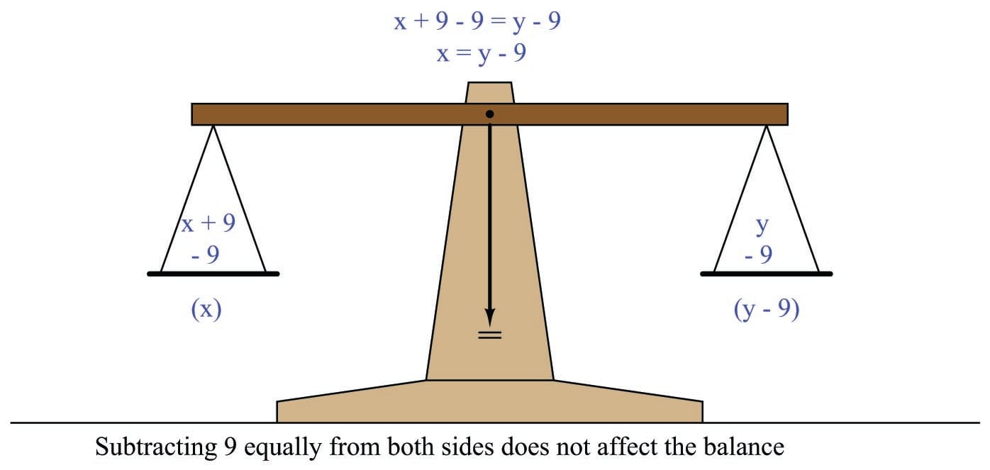
Returning to our expression \(x + 9 = y\), suppose we were tasked with solving for \(x\). In other words, we need to manipulate this equation to get \(x\) by itself on one side of the equals sign, with everything else on the other side of the equals sign. Clearly, the problem here is how to get rid of the “9” that’s being added to \(x\) on the left-hand side of the equation. One way to do this is to subtract 9 from both sides of the equation, thus canceling the “9” on the left-hand side and shifting it over to the right-hand side. This results in \(x\) being left all by itself on the left-hand side of the equation, just like we want:
Although we have the mathematical freedom to do anything we wish to both sides of the equation so long as we do it equally, we can see here that only one operation will work to isolate \(x\) by itself. This, therefore, is the challenge of algebraic manipulation: how to determine which operation(s) we should apply to both sides in order to end up with the equation re-written the way we want?
A general principle to help us answer this challenge is that of inverse functions: that is, pairs of mathematical operations known to “un-do” each other. The inverse function to addition is subtraction, which is why we subtracted 9 from each side of the equation \(x + 9 = y\) in order to “un-do” the addition of 9 to \(x\) on the left-hand side. In other words, we determine the mathematical operation being applied to the variable we wish to isolate, and then we intentionally apply the opposite mathematical operation to both sides of the equation to “strip away” that interfering operation.
Here is a table showing a few inverse mathematical functions:
| Function $f(x)$ | Inverse function $f^{-1}(x)$ |
|---|---|
| Addition (+) | Subtraction ($-$) |
| Multiplication ($\times$) | Division ($\div$) |
| Power ($x^n$) | Root ($\root n \of {x}$) |
| Exponent ($n^x$) | Logarithm ($\log_n x$) |
It should be noted that sometimes we can use the same function to “un-do” itself if we apply the quantity creatively. For example, instead of subtracting 9 from each side of the equation \(x + 9 = y\) to solve for \(x\), we could have just as easily added \(-9\) to both sides, which is mathematically equivalent. Likewise, instead of using division to “un-do” multiplication, we may simply multiply by the reciprocal, as in the following example where we wish to solve for \(x\) in the equation \({5 \over 3}x = y\). Since we can see that the fraction \(5 \over 3\) is being multiplied by \(x\), we may get rid of the fraction by multiplying both sides by its reciprocal (\(3 \over 5\)), leaving \(x\) multiplied by a factor of 1, which is the same as \(x\) all by itself:
\[{5 \over 3} x = y\]
\[\left({3 \over 5}\right) {5 \over 3} x = \left({3 \over 5}\right) y\]
\[{1 \over 1} x = \left({3 \over 5}\right) y\]
\[x = {3 \over 5} y\]
Had we chosen to divide both sides of this equation by the fraction \(5 \over 3\), we still would have arrived at a mathematically correct result, but it would have taken the form of a compound fraction, which is not as “elegant” a presentation:
\[{5 \over 3} x = y\]
\[{{5 \over 3} x \over {5 \over 3}} = {y \over {5 \over 3}}\]
\[x = {y \over {5 \over 3}}\]
The task of solving for a variable becomes more complicated when there are multiple operations needing to be stripped away to isolate a particular variable. Take for example the equation \(5x - 4 = y\), where we wish to solve for \(x\). Clearly, we must find a way to “un-do” the subtraction of 4, as well as the multiplication by 5, but which inverse operation should we apply first? The key here is to properly recognize the order of operations expressed in the original equation.
If we were to evaluate the equation \(5x - 4 = y\) to arrive at a value for \(y\) given a value for \(x\), our proper order of operations would be to first multiply \(x\) by 5, and then subtract 4. Multiplication/division precedes addition/subtraction, if there are no other influences such as parentheses. If our goal is to “un-do” each of these operations in order to arrive at \(x\) by itself, we must do so in reverse order of operations. This means first un-doing the subtraction of 4, and then un-doing the multiplication by 5. The following steps show how this is done:
| Step | Equation | Explanation |
|---|---|---|
| 1 | \(5x - 4 = y\) | Original equation |
| 2 | \(5x - 4 + 4 = y + 4\) | Adding 4 to both sides |
| 3 | \(5x = y + 4\) | Simplifying |
| 4 | \({5x \over 5} = {{y + 4} \over 5}\) | Dividing both sides by 5 |
| 5 | \(x = {{y + 4} \over 5}\) | Simplifying |
Note how these steps would have been different if the original equation were written with a different order of operations, such as \(5(x - 4) = y\). With the parentheses forcing the order of operations such that the subtraction occurs before the multiplication, our steps for isolating \(x\) must reverse as well – we must first divide by 5, then add 4:
| Step | Equation | Explanation |
|---|---|---|
| 1 | \(5(x - 4) = y\) | Original equation |
| 2 | \({5(x - 4) \over 5} = {y \over 5}\) | Dividing both sides by 5 |
| 3 | \(x - 4 = {y \over 5}\) | Simplifying |
| 4 | \(x - 4 + 4 = {y \over 5} + 4\) | Adding 4 to both sides |
| 5 | \(x = {y \over 5} + 4\) | Simplifying |
Linking formulae to solve mathematical problems
Most practical problems with mathematical solutions do not come to us with the proper formula pre-packaged for our use. Instead, we must identify relevant formulae relating the given variables together, and then use those formulae in combination to solve for the quantity we seek. The task of linking formulae to solve mathematical problems is one many students find quite challenging, and so it is worth our time to explore this in some detail.
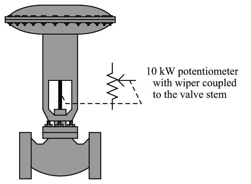
Example: sensing valve position
For our first example we will consider a scenario where we wish to have a computer sense the stem position of a control valve. A linear potentiometer coupled to the valve stem will provide us with a suitable sensor to convert the valve stem’s position into an electrical signal the computer can measure with appropriate analog I/O hardware:
This potentiometer may be used as one-half of a voltage divider network, with a constant-voltage power supply for the source, and a fixed resistor across which the computer’s analog I/O can read a voltage drop. As valve stem position changes, the potentiometer’s resistance in this circuit will change, thereby changing the voltage seen by the analog input module connected to the computer:
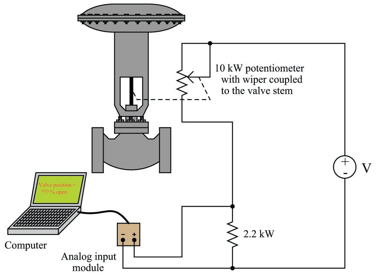
The problem we are now faced with is this: how do we program the computer to display the valve stem’s position in percent (on a 0% to 100% range), when all it directly senses from the circuit is a varying DC voltage? It certainly would not be helpful to have the computer display the raw signal in units of volts. What we need is a mathematical formula to translate that sensed voltage drop across the 2200 ohm resistor into a percentage value representing valve stem position.
Our first step needs to be identifying all the relevant mathematical formulae in this problem. Since the computer is sensing the voltage drop across one of two resistors in a series circuit, it would appear the voltage divider formula is relevant here (relating source voltage and circuit resistances to voltage drops):
\[V = V_{source}\left({R \over R_{total}}\right)\]
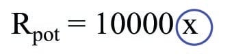
We also need to somehow relate the valve’s stem position (we’ll use \(x\) to represent the per unit value of valve opening) to the resistance of the potentiometer. If 0% stem position (i.e. \(x = 0\), valve fully closed) drives the potentiometer wiper fully down and 100% stem position (i.e. \(x = 1\), valve fully open) drives the wiper fully up, the potentiometer’s resistance in this circuit should be a simple proportion of its full 10000 ohm value:
\[R_{pot} = 10000 x\]
Now that we have a formula relating valve stem position to electrical resistance, and another formula relating electrical resistance to voltage drop, we are ready to link these two formulae together and derive a function expressing voltage drop as a function of valve stem position.
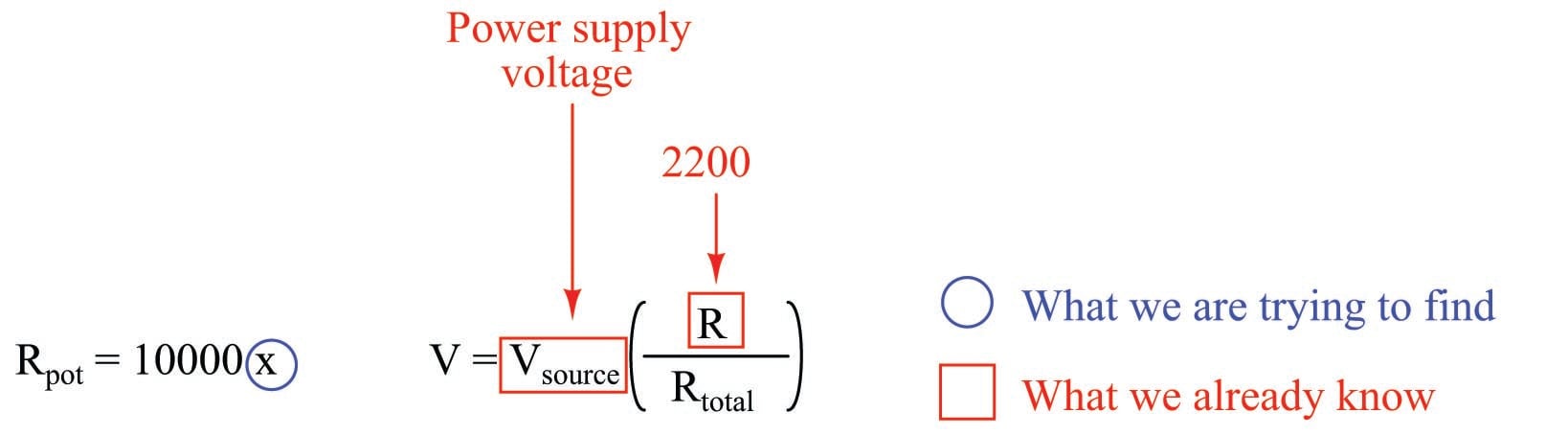
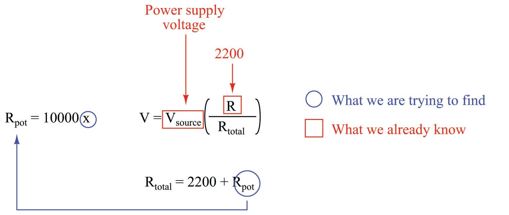
A useful strategy for identifying how multiple formulae link together is to “mark up” those formulae on paper to show how their variables relate to the given information as well as to each other. A standard I find easy to remember and apply is to draw a circle around the variable I’m need to solve the value of, and to draw a square or a rectangle around any variables whose values are given. To begin this process, I will write both the voltage divider and potentiometer proportion formulae near each other, then circle \(x\) (valve stem position, per unit) as the variable I need to solve for:
Of course, a basic rule of algebra is that for any one formula it is only possible to solve for the value of one variable. This means all other quantities in a formula must be known in order to solve for that one variable. In the \(R_{pot}\) formula we have \(x\) which we’re trying to solve the value of, the full-scale resistance value of 10000 ohms which is given to us in the problem, and the potentiometer’s manifested resistance value in the circuit (\(R_{pot}\)). Since 10000 is a constant, the only other piece of information we need in this formula to solve for \(x\) is the resistance value \(R_{pot}\). The fact that the variable \(R_{pot}\) remains unmarked makes this point clear: \(R_{pot}\) is the missing piece of the puzzle to solve for \(x\).
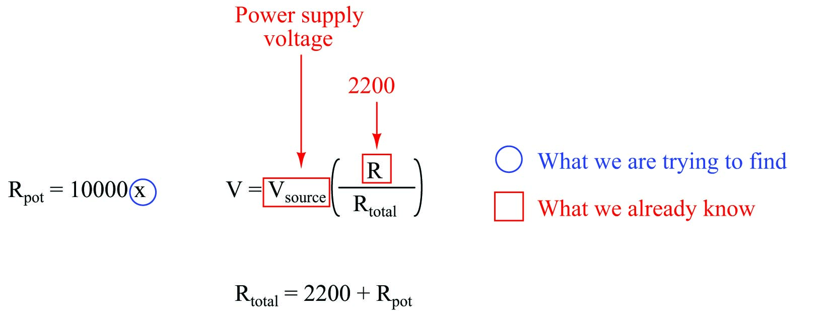
At this juncture we look to the other formula on hand to see if any of its variables will provide us this missing information. Here, it should be clear we need to find out where \(R_{pot}\) might fit in the voltage divider formula. The \(R\) variable in the numerator of the fraction in this formula refers to the resistance across which we are measuring the voltage drop \(V\). In this case, \(R\) must be the 2200 ohm fixed resistor, so we will enclose \(R\) in a square to represent the fact we know its value. Since the power supply’s voltage is constant, we may also enclose \(V_{source}\) in a rectangle to show that value will be available to us:
The only other resistance variable in the voltage divider formula is \(R_{total}\), which refers to the total resistance of the series-connected resistors in a voltage divider circuit. This particular circuit has two resistors: the 2200 ohm fixed resistor and the potentiometer. We know that total resistance in a two-resistor series circuit is the sum of those two resistors’ individual values (\(R_{total} = R_1 + R_2\)), we we will write this as a third formula in our collection, with \(R_1\) being the 2200 ohm fixed resistor and \(R_2\) being the potentiometer’s resistance:
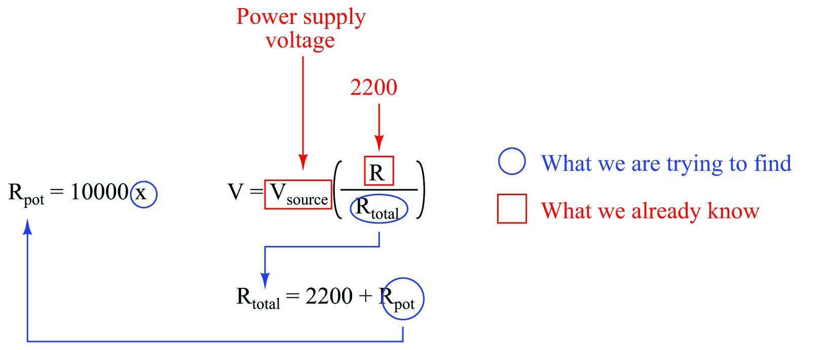
Now we are ready to link these formulae together. Recall how we needed to find the value of \(R_{pot}\) in the potentiometer’s formula before we could calculate the value of \(x\) (valve stem position). Note how the \(R_{total}\) formula relates that potentiometer resistance value to the other resistances in the circuit. This means the total resistance formula can provide us the value of \(R_{pot}\) we need to solve for \(x\). We will draw a circle around \(R_{pot}\) in the total resistance formula reminding us we need that value, then show a link between this and the potentiometer formula by drawing an arrow extending from one to the other:
So far, this markup tells us \(R_{pot}\) is the missing puzzle piece to calculate \(x\), and that \(R_{total}\) is the missing puzzle piece to calculate \(R_{pot}\).
Looking at our three formulae, we see that the voltage divider formula is able to provide us with the value of \(R_{total}\) which we need to calculate \(R_{pot}\) which we need to calculate \(x\). We will circle \(R_{total}\) in the voltage divider formula and draw another arrow showing the link:
The only variable unmarked and unlinked now is \(V\), which is the voltage sensed by the computer’s analog input module. This is now the one independent variable which will tell us the position of the valve stem (\(x\)).
Each arrow linking formulae together shows us where one formula will be substituted for a variable in another formula. The only thing we must do now prior to this substitution is algebraically manipulate each formula to solve for the one circled variable within it. I will skip these algebraic steps for brevity, and simply re-write the three formulae in manipulated form:
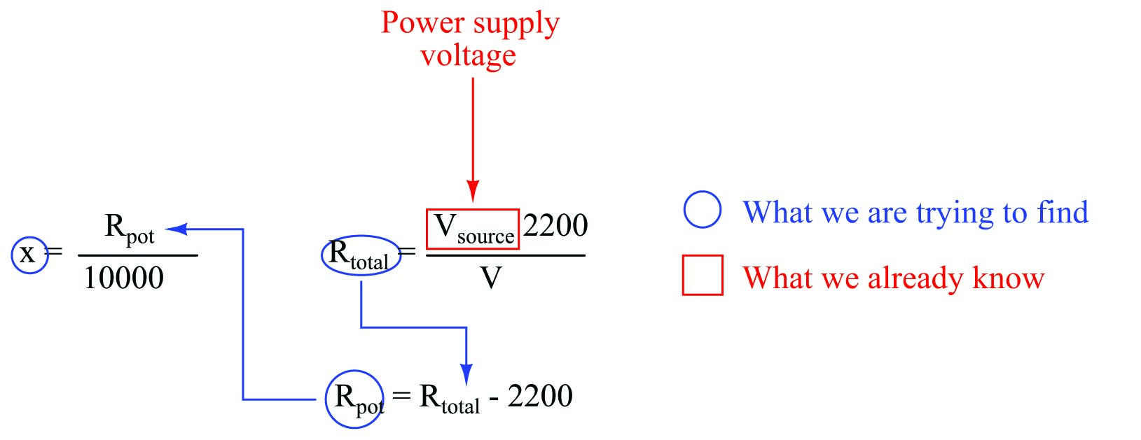
The logic chain of dependency linking these three formulae together is now crystal-clear: we begin with a measured voltage drop value of \(V\) to give us the value of \(R_{total}\), which then plugs into the total resistance formula to give us the potentiometer’s value \(R_{pot}\), which then plugs into the potentiometer formula to give us valve stem position (\(x\)) as a per unit value. The algebraic substitutions are shown here:
Substituting \(R_{total} - 2200\) for \(R_{pot}\) in the \(x = {R_{pot} \over 10000}\) formula:
\[x = {{R_{total} - 2200} \over 10000}\]
Substituting \(V_{source} 2200 \over V\) for \(R_{total}\) in the \(x = {R_{total} - 2200 \over 10000}\) formula:
\[x = {{{V_{source} 2200 \over V} - 2200} \over 10000}\]
This final formula can now be programmed into the computer, telling the computer how to calculate \(x\) as a function of \(V\).
To summarize this problem-solving strategy:
- Begin by writing every formula you can think of relevant to the problem at hand.
- Identify the final value you’re trying to solve for, and circle it.
- Identify all given values, and show them by drawing squares or rectangles around those variables.
- Identify any and all “missing puzzle pieces” in the formula with the circled variable.
- If there is another formula containing a “missing puzzle piece,” circle that variable and draw an arrow linking it to the previous formula, then identify any and all “missing puzzle pieces” needed to solve for that variable. There should only be one circled variable per formula.
- Repeat the previous step as often as needed until there are no missing pieces left.
- Algebraically manipulate all formulae to solve for their circled variables.
- Algebraically substitute all variables as shown by the arrows.
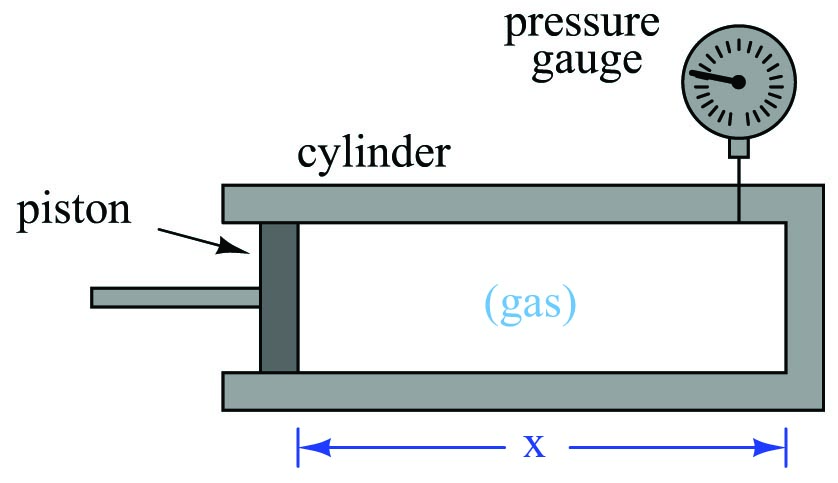
Example: gas pressure inside a cylinder
Let’s apply this technique to a practical problem related to engine and compressor mechanisms – how to determine the amount of gas pressure generated inside a cylinder when a piston is moved to compress the gas, given the distance of the piston’s motion (\(x\)):
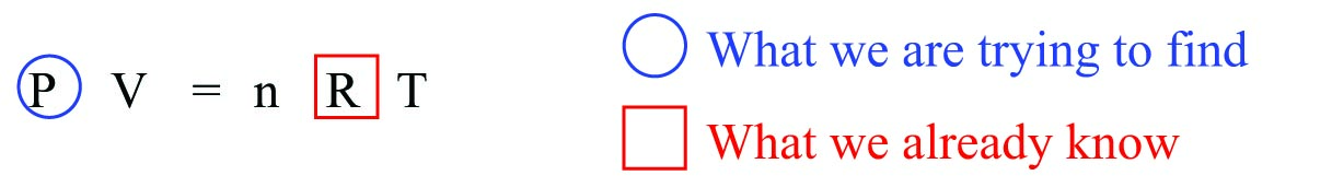
Compression is nothing more than a forced reduction in volume, and so a good first step for us to take is to recall any mathematical formulae relating pressure and volume for a confined gas. In this case, the Ideal Gas Law is our clear choice, describing the relationship between gas pressure, volume, temperature, and the molar gas quantity inside any enclosed volume:
\[PV = nRT\]
Where,
\(P\) = Absolute pressure (atmospheres)
\(V\) = Volume (liters)
\(n\) = Gas quantity (moles)
\(R\) = Universal gas constant (0.0821 L \(\cdot\) atm / mol \(\cdot\) K)
\(T\) = Absolute temperature (K)
However, the Ideal Gas Law formula contains no variable \(x\) to represent piston position. Somehow, we must find a way to relate \(x\) to the Ideal Gas Law formula in order to progress to a solution for this problem.
The first step in applying this formula is to identify which variables are given to us in the problem, and which we need to solve for. In order to solve for the value of any one variable in an equation, there cannot be any other unknown quantities – this is a basic law of algebra.
In this case, the variable we’re ultimately trying to solve for is pressure (\(P\)). The only other quantity found in the Ideal Gas Law formula that we know the value of at this point is \(R\), which is a natural constant. \(V\), \(n\), and \(T\) are all unknown to us at this point in time. Once we do know the values of these three variables, we may algebraically manipulate the Ideal Gas Law formula to solve for \(P\).
Once again we will begin by “marking up” the formula by drawing a circle around the variable we wish to solve for, and drawing squares around any variables or constants for which we already know the values. Any variables left unmarked (i.e. not enclosed in a circle or a square) are unknown quantities which we must determine before we can solve for the circled variable:
This first step of identifying known and unknown quantities is critically important to the process of problem-solving, because it directs us to what we need to do next. An obstacle so many students and professionals alike experience is paralysis in problem-solving: they get part-way into solving a problem and encounter a point where they have no idea what to do or where to go next. This is why having a strategy to identify the next step is so vitally important.
After identifying these unknown variables of \(V\), \(n\), and \(T\), we now know we need to either find other formulae to solve for those values, or investigate the real mechanism to see if we may directly measure their values.
It should be clear that temperature (\(T\)) is one of those variables we should be able to directly measure in the mechanism. We know in order to solve for pressure (\(P\)) given piston position (\(x\)), one of the real-world parameters we must first measure is temperature.
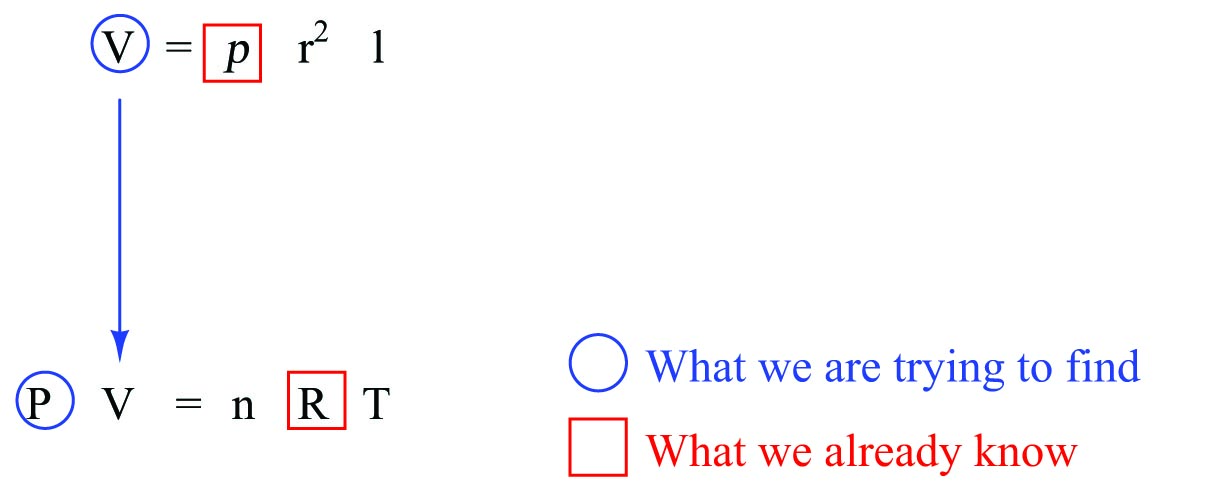
It should also be clear that volume (\(V\)) is a variable related to piston position (\(x\)), and as such we should be able to identify a formula relating the two, which we may then combine with the Ideal Gas Law formula to arrive at one step closer to our solution. Since the interior volume of the machine’s cylinder is, well, cylindrical, we know that the formula for calculating the volume of a cylinder is what we need to incorporate next:
\[V = \pi r^2 l\]
Where,
\(V\) = Volume of cylinder
\(\pi \approx\) 3.1415927
\(r\) = Radius of cylinder
\(l\) = Length of cylinder
As we did with the Ideal Gas Law formula, our next step is to identify in the cylinder volume formula those quantities we currently know versus those we don’t (and therefore those we need to find). Marking up the formula with circles and squares is helpful, as is drawing an arrow between the variable we’re trying to solve for with the cylinder formula and where it goes in the Ideal Gas Law formula. This arrow visually links the two formulae together, showing us where we will eventually need to perform algebraic substitution:
Pi (\(\pi\)) of course is a natural constant, just like \(R\), so we enclose it in a square to show that we know its value. \(r\) is the radius of the cylinder, which in the mechanism’s case is the same as the radius of the piston. As with temperature, this is a quantity we will need to determine in order to solve this problem. Length (\(l\)) is exactly the same as the piston position given to us in the problem: \(x\), meaning we may re-write the cylinder volume formula as \(V = \pi r^2 x\). Representing all of these relationships graphically:
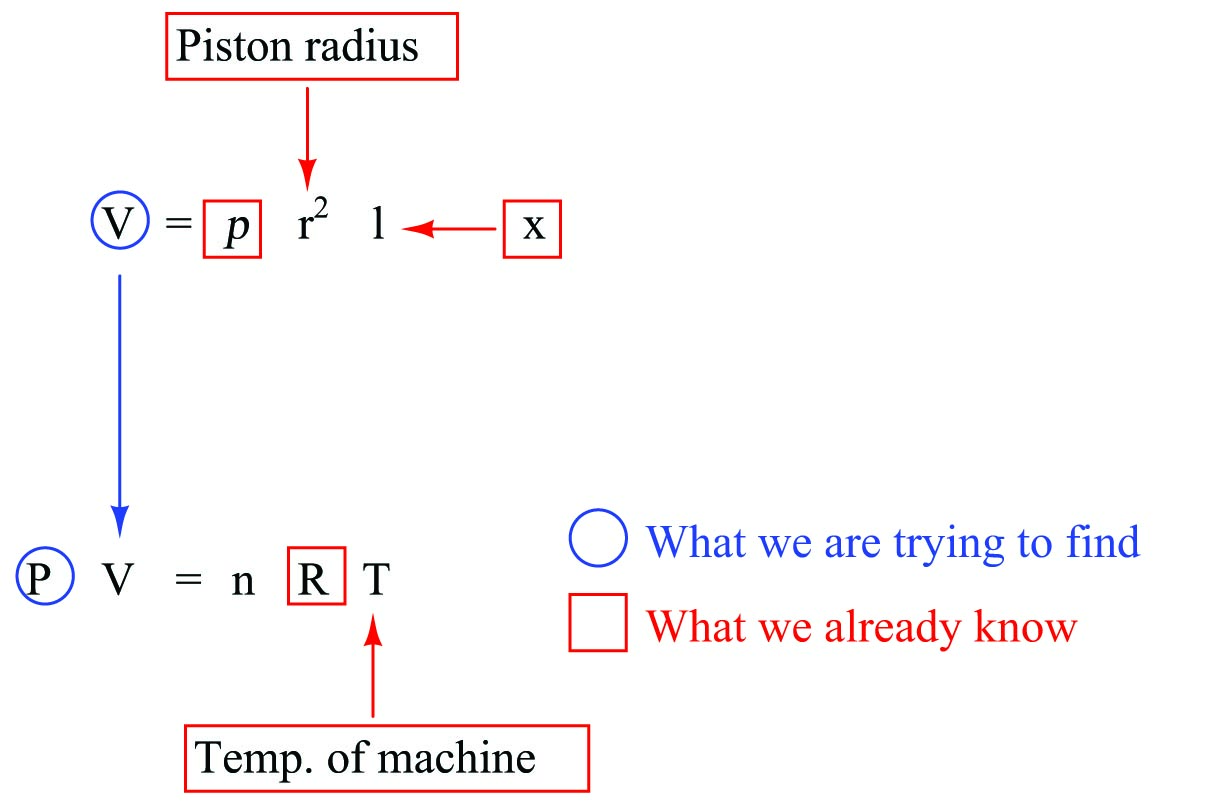
The only unknown still existing is \(n\), the number of moles of gas held inside the cylinder. This is not something one would be able to directly measure, like temperature, piston radius, or piston position. Either this is a quantity that would have to be provided to us as a given condition in the problem, or we must know something else about the problem in order to find the value of \(n\). We will set aside this issue for the time being and concentrate for now on how to combine the cylinder and Ideal Gas Law formulae.
As our graphical markup of the two formulae show us, volume (\(V\)) calculated by the cylinder formula is what gets “plugged in” to the Ideal Gas Law formula (\(V\) as well). In algebra, this operation is called substitution: replacing a single variable in an equation with another equation.
\[\hbox{Substituting} \hskip 10pt V = \pi r^2 x \hskip 10pt \hbox{for} \hskip 10pt V \hskip 10pt \hbox{in} \hskip 10pt PV = nRT \hskip 10pt \hbox{. . .}\]
\[PV = nRT\]
\[P (\pi r^2 x) = nRT\]
\[P \pi r^2 x = nRT\]
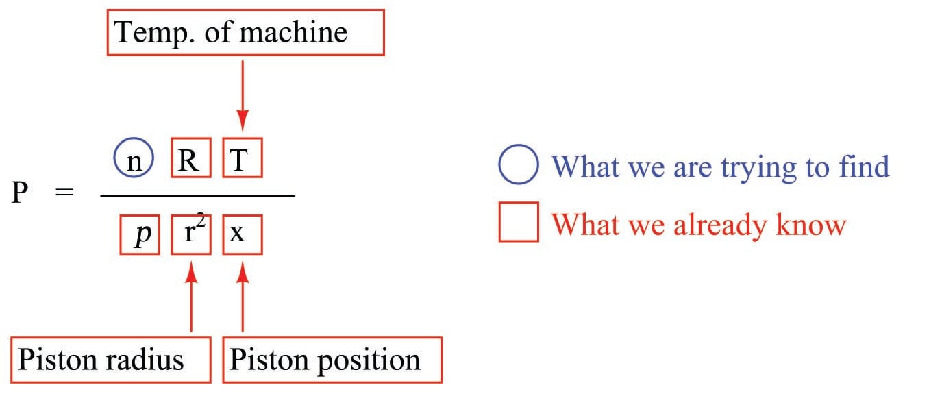
\[\hbox{Now, solving for} \hskip 10pt P\]
\[P = {{n R T} \over {\pi r^2 x}}\]
We now have a formula for \(P\) written as a function of \(x\). Provided we know the temperature (\(T\)), the piston’s dimensions, and the molecular quantity of gas inside the cylinder (\(n\)), we may plug any arbitrary value for piston position (\(x\)) and very easily calculate pressure (\(P\)).
Returning to the question of knowing the value of molecular gas quantity (\(n\)), we might ask ourselves, “What if no one provided us with a value for \(n\)? How could we possibly solve for pressure then?” Recall once more the basic law of algebra telling us we can only solve for one unknown quantity in a single equation at one time. What would we need to know in our custom formula in order to solve for \(n\)? A graphic markup of the formula is helpful once again:
From this we can see it would be possible to calculate \(n\), if only we knew \(P\). Clearly, this is a Catch-22: our goal is to calculate the value of \(P\) from \(n\), yet the only algebraic means we have of determining \(n\) is to first know the value of \(P\).
However, there is a solution to this conundrum. Most engine and compressor mechanisms work by moving the piston back and forth in coordination with valves to vent and direct the flow of gas into and out of the cylinder. This usually means there will be other piston positions where vent valve(s) are open to ensure atmospheric pressure inside the cylinder. In other words, there will be other values of \(x\) for which the pressure \(P\) will be known. In such a case where both \(x\) and \(P\) are known, we may solve for \(n\), and then be confident that value of \(n\) will be the same for other piston positions because the vent valves close off before compression begins, trapping all gas molecules inside the cylinder.
Representing two such conditions, using subscripts to distinguish pressures and piston positions in each of the two conditions. Here, we will assume that the gas temperature is the same in both conditions, to simplify the problem:
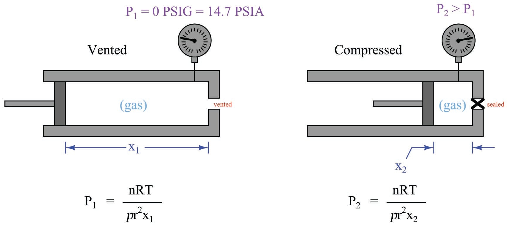
Now that we have a means to solve for \(n\), we may use substitution again to replace \(n\) in the “compressed” formula (condition 2) with the \(n\) from the “vented” formula (condition 1). A key assumption in making this substitution is that we know \(n\) will actually be the same value for those two conditions, which is a safe assumption because compression machines seal off the cylinder (preventing gas entry or escape) prior to the compression stroke of the piston.
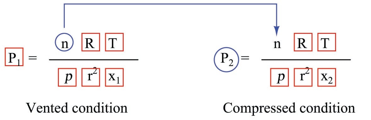
To do this substitution, we must first manipulate the first equation to solve for \(n\), then replace \(n\) in the second equation with our manipulated first equation:
\[P_1 = {nRT \over \pi r^2 x_1}\]
\[n = {\pi r^2 x_1 P_1 \over RT}\]
\[\hbox{Substituting . . .} \hskip 10pt n\]
\[P_2 = {\left({\pi r^2 x_1 P_1 \over RT}\right) RT \over \pi r^2 x_2}\]
Here we see something very interesting: following the substitution, many of the variables and constants cancel each other out, leaving us with a much simpler formula solving for \(P_2\) in terms of \(x_1\) and \(x_2\). First, we cancel \(RT\) out of the numerator:
\[P_2 = {\left({\pi r^2 x_1 P_1 \over RT}\right) RT \over \pi r^2 x_2}\]
\[P_2 = {\pi r^2 x_1 P_1 \over \pi r^2 x_2}\]
Next, we cancel out \(\pi r^2\) from numerator and denominator:
\[P_2 = {x_1 P_1 \over x_2}\]
\[P_2 = {x_1 \over x_2} P_1\]
Thus, the machine’s gas pressure in the compressed condition is a simple ratio of its two piston positions multiplied by the absolute pressure in the vented condition.
Double-checking calculations
When performing calculations to arrive at an answer to some problem, it is important to check your work. Even if all the algebraic work you’ve done is perfectly correct, it is still possible to commit simple “keystroke” errors while entering numbers or executing operations on your calculator, and/or to make simple mental-math calculation errors. For this reason, teachers from time immemorial have encouraged their students to double-check their work.
What many students tend to do, unfortunately, is check their work by following all the same steps one more time and seeing if they get the same answer as before. While this might make sense to do at first, it actually invites the exact same errors, because our short-term memory for calculator keystrokes and mental math operations tends to be quite good. If we made a keystroke error the first time, we are very likely to make the exact same keystroke error the second time, simply following muscle memory.
A good way to avoid this error is to check your mathematical work backwards, beginning with the answer you previously calculated, working backwards through the equations to see if you can arrive at one of the values given to you at the start of the problem. This technique forces you to approach the problem differently, using different keystrokes in different orders.
For example, suppose you were tasked with calculating the pressure generated by a vertical column of liquid inside a process vessel, in order to properly set the lower- and upper-range values (LRV and URV) for the hydrostatic level transmitter:
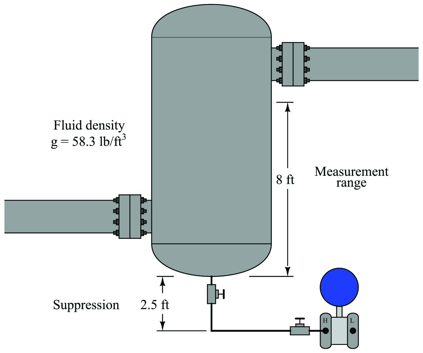
The pressure seen by the transmitter at a 0% level condition (empty vessel) should be only that produced by the 2.5 foot height of the impulse tubing filled with process fluid:
\[P = \gamma h\]
\[P = (58.3 \hbox{ lb/ft}^3)(2.5 \hbox{ ft})\]
\[P = 145.75 \hbox{ lb/ft}^2 = 1.012 \hbox{ PSI}\]
Likewise, the pressure seen by the transmitter at a 100% level condition should be that produced by the impulse tubing height and the vessel’s internal fill of 8 feet:
\[P = \gamma h\]
\[P = (58.3 \hbox{ lb/ft}^3)(2.5 \hbox{ ft} + 8 \hbox{ ft})\]
\[P = (58.3 \hbox{ lb/ft}^3)(10.5 \hbox{ ft})\]
\[P = 612.15 \hbox{ lb/ft}^2 = 4.251 \hbox{ PSI}\]
If we wished to check our final answer of 4.25 PSI, we could work backwards from this result to try to calculate the total fluid height of 10.5 feet, or work backwards to calculate the fluid density of 58.3 lb/ft\(^{3}\). Let’s do the latter and see what we get:
\[\gamma = {P \over h}\]
\[\gamma = {612.15 \hbox{ lb/ft}^2 \over 10.5 \hbox{ ft}}\]
\[\gamma = 58.3 \hbox{lb/ft}^3\]
Although this technique may seem obvious, it nevertheless avoids the pitfalls of repeating keystroke errors, which is an error plaguing the work of many students!
A variation on this theme is to calculate a quantity not given or reached in any of the initial problems. Here, for example, we were tasked with determining the transmitter’s lower- and upper-range values (pressures at 0% fill and 100% fill). One way to check our work is to see if a different fill condition such as 50% gives us a pressure value lying exactly half-way between the LRV of 1.012 PSI and the URV of 4.251 PSI.
If we imagine the vessel half-full, our total liquid height seen by the transmitter will be 4 feet plus the suppression value of 2.5 feet, or 6.5 feet total. Calculating hydrostatic pressure at this liquid height:
\[P = \gamma h\]
\[P = (58.3 \hbox{ lb/ft}^3)(2.5 \hbox{ ft} + 4 \hbox{ ft})\]
\[P = (58.3 \hbox{ lb/ft}^3)(6.5 \hbox{ ft})\]
\[P = 378.95 \hbox{ lb/ft}^2 = 2.632 \hbox{ PSI}\]
A simple way to check that 2.632 lies half-way in between 1.012 and 4.251 is to calculate the average value of 1.012 and 4.251:
\[{{1.012 + 4.251} \over 2} = 2.632\]
Sure enough, it checks out to be correct. This is good validation of our initial work in calculating the transmitter’s LRV of 1.012 PSI and URV of 4.251 PSI.
Yet another variation on this same theme of checking your work different ways is to approach the problem differently altogether. We know we may calculate the LRV and URV pressure values for this process vessel and fluid if we convert the fluid’s density into a specific gravity value (58.3 lb/ft\(^{3}\) = 0.9339) and then calculate hydrostatic pressure as though we were dealing with inches water column, corrected for the specific gravity of this process fluid.
A height of 2.5 feet (0% level) is 30 inches, which when multiplied by the specific gravity value of 0.9339 yields 28.016 inches WC, which is equivalent to our first calculated pressure value of 1.012 PSI.
A height of 10.5 feet (100% level) is 126 inches, which when multiplied by the specific gravity value of 0.9339 yields 117.67 inches WC, which is equivalent to our first calculated pressure value of 4.251 PSI.
As you can see, solving for LRV and URV pressures using an entirely different technique yields the same answers as before, which is good validation of our original work.
It is important to note that double-checking your work in this manner merely helps confirm your original work, but it does not conclusively prove your original answers are correct. For example, one of the numbers we keep using in the URV calculations is the total liquid height of 10.5 feet. Suppose, though, that this height value was something we incorrectly calculated mentally by adding the suppression and the range heights. For example, suppose our actual given heights in the problem were a 2.5 feet suppression height and a 7 foot measurement range, and we mistakenly added 2.5 feet and 7 feet in our heads to get 10.5 feet. If that were the case, both the original URV pressure calculation and the subsequent double-checks might still agree with one another, but could still be wrong because they all depend on that same 10.5 foot height value.
The most realistic attitude to maintain in all problem-solving is scientific skepticism: there is no such thing as absolute proof so long as the potential for error exists. Given that you are a human being – liable to all manner of fallacies and mistakes – absolute proof will forever lie outside your grasp. The best we can do is incrementally minimize the potential for errors and mistakes, and accept the inevitable uncertainty.
Maintaining relevance of intermediate calculations
A very common attitude I’ve noticed with students is something I like to call “any procedure, so long as it works.” When learning to solve particular types of quantitative problems, the natural tendency is to identify procedural techniques for calculating the correct answer(s), and then practice those procedures until they can be performed without flaw. Unfortunately, it is all too easy to lose focus on principles when the learning emphasis is on procedure. The allure of a procedure guaranteed to yield correct answers overshadows the greater need to master and apply fundamental principles, leading to poor problem-solving ability masked by an illusion of competence.
This is a significant obstacle to deep and significant learning in the sciences, and there is no one solution to it. However, there is a way to identify and self-correct this behavior in some contexts, and it relies on a habit of identifying the real-world relevance of all intermediate calculations within a quantitative problem.
To illustrate, let us consider a simple voltage divider circuit comprised of two resistors, where some amount of supply voltage is divided into a smaller proportion to become the output voltage signal. The problem at hand is calculating the output voltage of this divider circuit, knowing the values of supply voltage and resistor resistances:
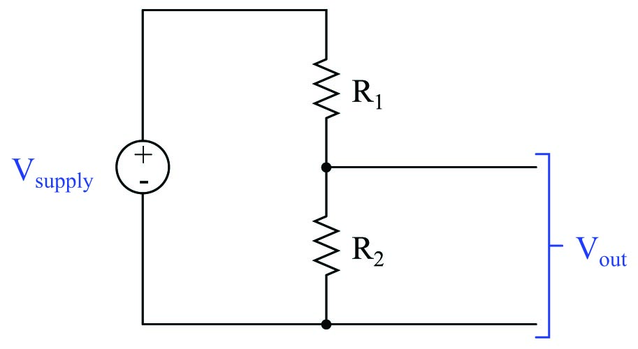
One of the basic formulae all beginning electronics students learn is the appropriately named voltage divider formula, shown here:
\[V_{out} = V_{supply} \left( {R_2 \over R_1 + R_2} \right)\]
Calculating \(V_{out}\) is a simple matter of substituting known values of voltage and resistance into this formula, then performing the necessary arithmetic. However, the procedure by which a student evaluates this formula – particularly in regard to the understanding of fundamental concepts – matters greatly to that student’s mastery of circuit analysis.
Suppose a student evaluates the voltage divider formula according to the order of operations enforced by the parentheses. Note the sequence of steps in this procedure, and how each step yields a value relevant to the voltage divider circuit:
| Step | Calculation | Unit of measurement & Meaning | |
|---|---|---|---|
| 1 | $R_1 + R_2$ | Ohms | Total circuit resistance ($R_{total}$) |
| 2 | $R_2 \div R_{total}$ | (unitless) | Voltage division ratio |
| 3 | $V_{supply} \times \hbox{ Ratio}$ | Volts | Output voltage ($V_{out}$) |
Now let us suppose a student calculates the exact same output voltage for this divider circuit using a modified version of the voltage divider formula. This formula may be derived from the original version by applying the commutative property of multiplication, simply swapping the positions of \(R_2\) and \(V_{supply}\):
\[V_{out} = R_2 \left( {V_{supply} \over R_1 + R_2} \right)\]
The proper order of operations for this modified formula will be different from the original version, but the final result (\(V_{out}\)) will be identical. Each step of the evaluation still yields a value relevant and applicable to the voltage divider circuit:
| Step | Calculation | Unit of measurement & Meaning | |
|---|---|---|---|
| 1 | $R_1 + R_2$ | Ohms | Total circuit resistance ($R_{total}$) |
| 2 | $V_{supply} \div R_{total}$ | Amps | Circuit current ($I$) |
| 3 | $R_2 \times I$ | Volts | Output voltage ($V_{out}$) |
Finally, let us suppose a student calculates the exact same output voltage for this divider circuit using another modified version of the voltage divider formula. This formula may be derived from the original version by applying the associative property of multiplication, grouping \(R_2\) and \(V_{supply}\) together into the denominator of the fraction:
\[V_{out} = {R_2 V_{supply} \over R_1 + R_2}\]
The proper order of operations for this modified formula will be different from the original version, but the final result (\(V_{out}\)) will be identical. Note, however, the irrelevance of the result in step #2:
| Step | Calculation | Unit of measurement & Meaning | |
|---|---|---|---|
| 1 | $R_1 + R_2$ | Ohms | Total circuit resistance ($R_{total}$) |
| 2 | $R_2 \times V_{supply}$ | Volt-ohms | ??? |
| 3 | $R_{total} \times \hbox{ previous result}$ | Volts | Output voltage ($V_{out}$) |
Despite the mathematical equivalence of this last formula to the prior two, step #2 makes no conceptual sense whatsoever. The product of resistance and voltage, while mathematically useful in solving for \(V_{out}\), has no practical meaning within this or any other circuit.
Conceptual problem-solving is an important skill, because it is only by mastering fundamental concepts can one become proficient in solving any arbitrary problem involving those concepts. Procedural problem-solving is useful only when applied to the specific type of problem the procedure was developed for, and useless when faced with any other type of problem. A student who understands the meaning of each step as they evaluate a voltage divider circuit will have little problem solving for quantities in other electrical circuits. A student who has merely memorized a step-by-step procedure for evaluating a voltage divider will struggle trying to solve for quantities in other circuits, unless they happen to have memorized step-by-step procedures for all those other circuits as well.
Troubleshooting is also closely linked with conceptual understanding. In my years as an instructor of electronics and instrumentation, I have seen an almost perfect correlation between conceptual understanding and diagnostic proficiency: procedural thinkers are invariably poor troubleshooters, and poor troubleshooters are invariably procedural thinkers.
The practical lesson we may draw from this example of voltage divider circuit evaluation is the importance of identifying the meaning of every intermediate result. If you ever find yourself performing calculations, unable to explain the practical significance of every step you take, it means you are thinking procedurally rather than conceptually. Instructors may apply this standard to their students’ work by asking students to explain the meaning of each and every calculation they perform.
