 Facebook
 Google
 GitHub
 Linkedin
General Problem-solving Techniques
A variety of problem-solving techniques have been presented for students over the years which are all helpful in tackling problems both in the classroom and in the real world. Several of these techniques are presented here in this section.
Identifying and classifying all “known” conditions
An important step in solving certain types of problems, especially quantitative problems where calculations are necessary to obtain precise answers, it is often useful to list all the known quantities available to us relevant to the problem. Similarly, taking the time to list all relevant (and possibly relevant) mathematical formulae we might apply to the solution is a helpful step.
One way to save time applying the latter suggestion in a classroom setting is to keep a concise reference card or file filled with formulae you’ve been learning within that course. This reference may be referred to as often as necessary, without having to re-write the equations for each and every problem, thus eliminating unnecessary effort.
Re-cast the problem in a different format
Many people find it easier to grasp the nature of a problem – and by extension, that problem’s solution – if they can look at an illustration of the problem. Therefore, a helpful step in solving problems described to you in words is to translate those words into a picture to look at.
If you are one of those people for whom drawing is a challenge, take heart in the fact that this is a skill you can build. Practice is the key to honing this skill. With this in mind, make it a habit to sketch some kind of illustration for every problem you are asked to solve. If you are working in teams to solve a problem, a collaborative sketch goes a long way toward coordinating problem-solving efforts and ensuring everyone on the team has the same view of the problem.
For some people, describing a problem verbally is helpful in solving it. If your brain tends to work like this – understanding concepts and situations better when they are cast into clear prose – then you may find it helpful to first draft an explanatory paragraph of the problem in your own words. This is also an exercise lending itself well to team-based problem solving, as the entire team can help each other describe the nature of the problem.
Working backwards from a known solution
Sometimes we may gain insight into the solution of a problem by assuming we already know the answer to a similar problem, then working “backward” to find the problem from that assumed solution.
An application of this problem-solving strategy is found learning how to decode binary bits that have been encoded using the Manchester standard. With Manchester encoding, binary bits are represented by the rising and falling edges of square-shaped waveforms rather than high and low states themselves. For example:
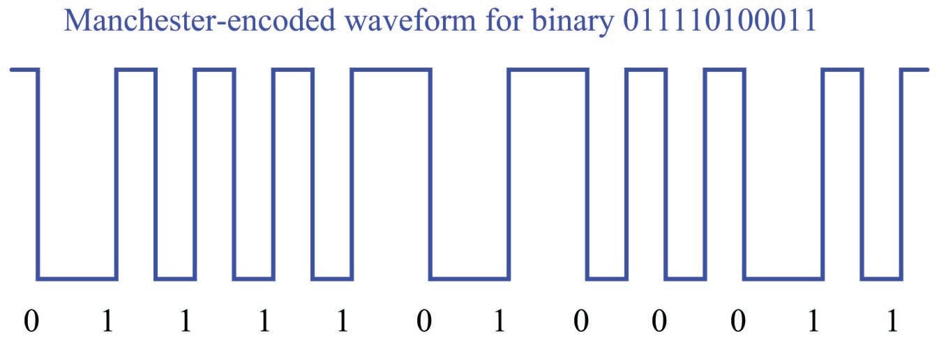
Seeing this example, we note how each binary “0” bit is represented by a falling edge, while each “1” bit is represented by a rising edge.
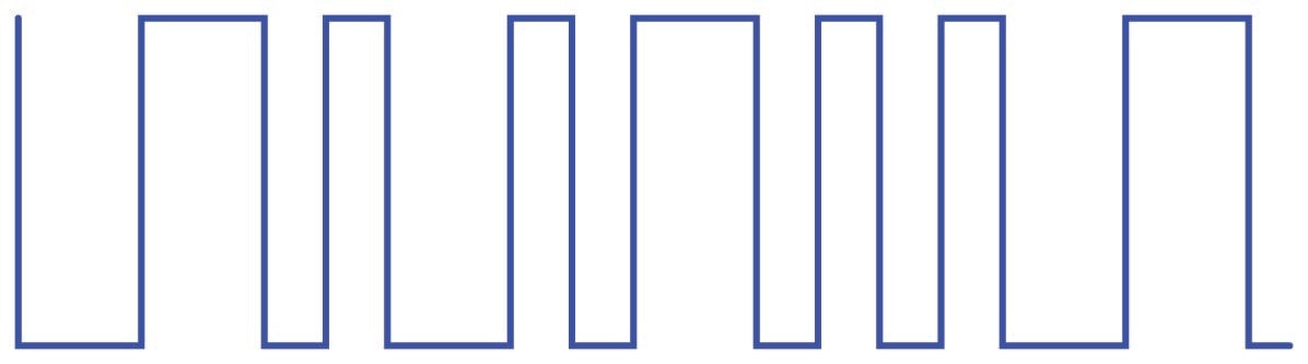
Where most students encounter trouble is in situations where they have been given a Manchester encoded waveform and must decode it into its representative bit stream. Take this for example:
Most students’ first inclination is to ask their instructor or their classmates for an algorithm to decode the waveform. “What steps should I take to figure out where the data bits are?” they will ask. This sort of “give me the answer” mind-set should always be discouraged, because it is the polar opposite of true problem-solving technique, where the student methodically searches for patterns and develops algorithms on their own.
A better approach is to encourage the strategy of working the problem backwards: begin with a known series of binary bits, and then develop a Manchester waveform from that. The act of encoding a binary string provides insight that will be useful in decoding the next Manchester waveform they encounter.
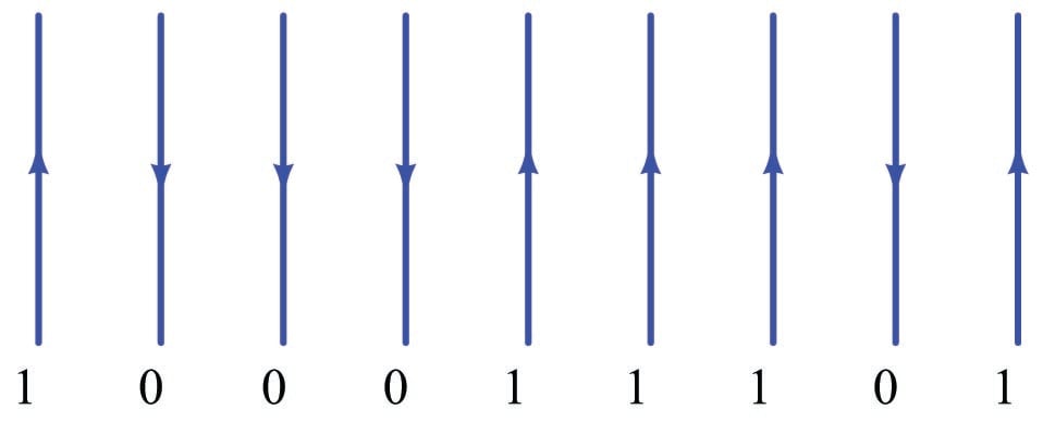
For example, let’s begin with the binary string 100011101:

We may begin the process of encoding this into Manchester format by sketching the rising- and falling-edges we know we will need for each bit:
Next, we can try connecting the tops and bottoms of these pulse edges to form a complete waveform. Soon, however, we will find that this is only possible where opposite bit states are adjacent to each other. Where identical bits follow in sequence, we are faced with sequential rising edges or sequential falling edges, which we cannot simply bridge at the tops or bottoms to make a full pulse:
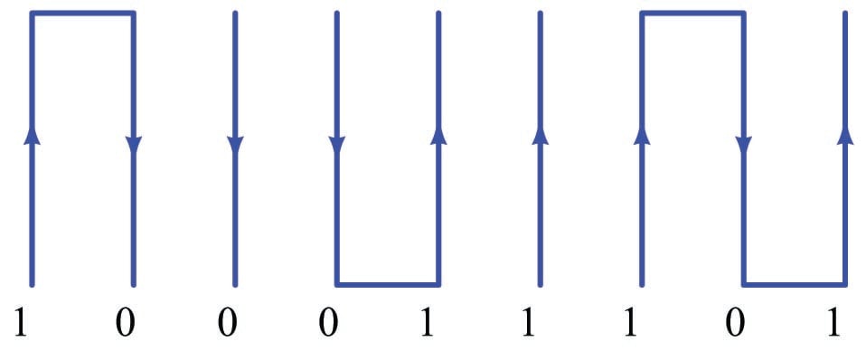
This observation leads to the realization of why we need reversals in a Manchester waveform. The only way to connect repeating bits’ edges together is if the waveform goes through another rising or falling edge in order to be properly set up for the next edge we need to represent a bit:
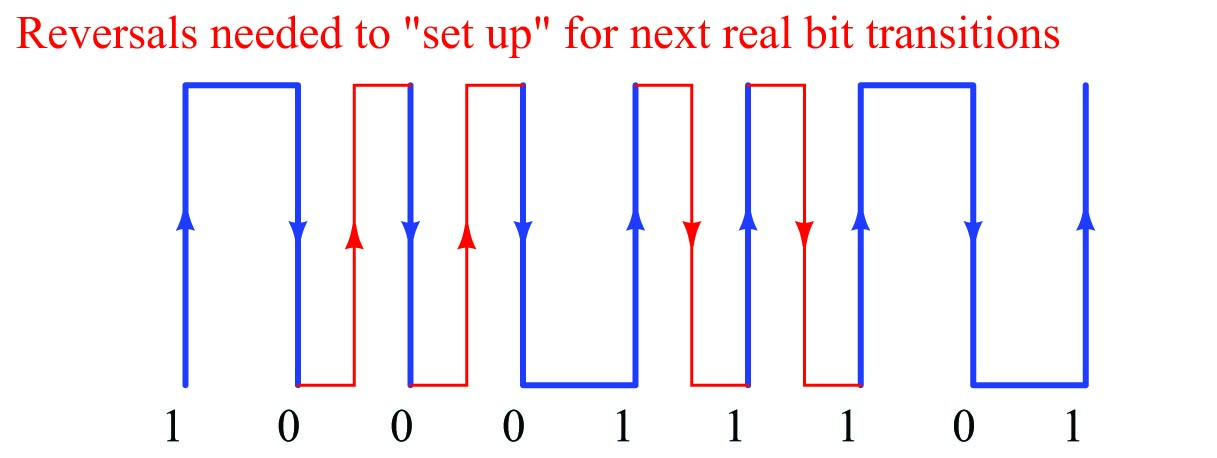
Here we see the power and utility of working a problem “backwards”: it reveals to us the reason why things are the way they are. Without this understanding, problem-solving is nothing more than rote recall of algorithms, and limited in application. Any problem becomes simpler to solve once we fully understand its rationale.
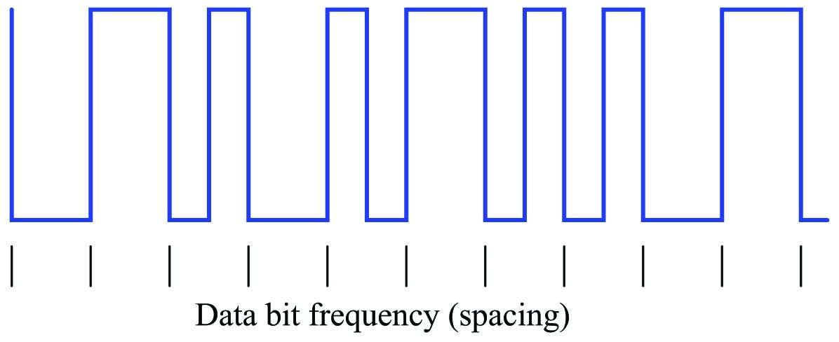
Once we realize the purpose for reversals in a Manchester waveform, it becomes obvious to see that these reversals always fall between the bit transitions, and thus are always out of step with the frequency of the bits. Those edge transitions representing real data bits must always fall along a regular timed interval, with reversals being “half-steps” in between those intervals. We need only to look for the widest-spaced intervals in a Manchester waveform to distinguish those pulse edges representing real data bits, and then we know to ignore any pulse edges out of step with them.
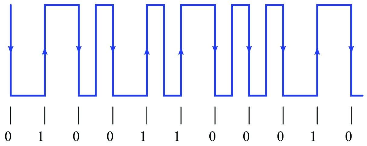
Returning to our sample problem, where we were given a Manchester waveform and asked to decode it:
First, we identify the real data bit edges by widest spacing:
Now that we know which pulse edges represent bits, we may ignore those that do not (the reversals), and decode the waveform:
Using thought experiments
One of the most powerful problem-solving techniques available for general use is something called a thought experiment. Scientists use experiments to confirm or refute hypotheses, testing their explanations by seeing whether or not they can successfully predict the outcome of a certain situation by comparing their predictions against real outcomes. While this technique is extremely useful, it might not always be practical or expedient. A useful alternative to real experiments is to mentally “model” the system and then imagine changing certain elements or variables within that model to deduce the effects.
Albert Einstein famously applied “thought experiments” to the formulation of his Theory of Relativity, for the very simple reason that he lacked the resources and technology to actually test his ideas in real life. Working as a patent clerk, he would imagine what might happen if an observer were to travel at or near the speed of light. One particular example of this is the anecdote of Einstein observing a clock tower as he rode a trolley traveling away from the tower. “What would an observer see,” he wondered, “as he viewed the clock’s face while traveling away from it at the speed of light?” Concluding that the clock’s face would appear to be frozen in time was one of the surprising “experimental” results leading Einstein to a more rigorous examination of physical effects at extremely high velocities.
“Thought experiments” are useful in solving a wide variety of problems, because they allow us to test our understanding of a system’s behavior. By imagining certain conditions or variables changing in a system and then asking ourselves what the effects will be, we probe our own understanding of that system, often times with the result being that we are able to predict its behavior under conditions that baffle us at first.
You will find “thought experiments” scattered throughout this book, used both as illustrations of problem-solving strategies and also as a tool to explain how certain technologies function. An example of this is the section explaining non-dispersive analyzers, which are instruments employing the absorption of light by certain species of chemicals in order to detect the presence and measure the quantities of those chemicals. Beginning in section 23.6 on page , a series of “thought experiments” are used to explore the principles used to identify chemicals by light absorption. This series of virtual experiments becomes most valuable when this section explores the analyzer’s ability to selectively measure the presence of one light-absorbing chemical to the exclusion of other light-absorbing chemicals within the same mixture.
Explicitly annotating your thoughts
Suppose you were asked to solve this multiplication problem, without the use of a calculating machine of any kind, but with access to paper and a writing tool:
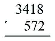
Your primary school education should have prepared you to solve elementary arithmetic problems of this kind, by a process of digit-by-digit multiplication and addition, to arrive at an answer of 1,955,096. The procedure, while tedious, is rather simple: manually multiply the top numeral three times over by successive digits of the bottom numeral, noting any “carried” quantities as you do so, then sum those three subtotals together (padded with zeros to represent the place of the bottom numeral’s digit) to arrive at the final product.
Now suppose you were asked to solve the exact same multiplication problem, but this time doing the same digit-by-digit arithmetic all in your mind, without the use of a writing tool to annotate your work. Suddenly this elementary task becomes nearly impossible for anyone who isn’t a mathematical savant. What made the difference between this problem as an elementary exercise and this same problem as a nearly impossible feat? The answer to this question is short-term memory: most people do not possess a good enough short-term memory to mentally manage all the intermediate calculations necessary to complete the calculation. This is why people learn to annotate their work when performing manual multiplication, so they don’t have to rely on their limited short-term memories. The freedom to write your steps on paper converts what would otherwise be a Herculean feat of arithmetic into a rather trivial exercise.
Annotating your intermediate steps as you solve a problem is actually an excellent general problem-solving strategy, applicable to far more than just arithmetic. Some examples of annotating intermediate steps are listed here:
- Reading a complex document: annotating your thoughts, questions, and epiphanies as you read the text allows you to derive a better understanding of the text as a whole.
- Learning a new computer application: noting how features are accessed and identifying the necessary conditions for each feature to work helps you navigate the software more efficiently.
- Following a route on a map: marking where you started, where your destination is, and where you have traveled thus far helps you see how far you still need to go, and which alternative routes are open to you.
- Analyzing an electric circuit: annotating all calculated voltages, currents, and impedances on the diagram helps you keep track of what you know about the circuit and where to go next in your analysis.
- Troubleshooting a system fault: noting all your diagnostic steps and conclusions along the way helps you confirm or disprove hypotheses.
Sadly, many students attempt to solve new types of problems analogously to performing multiplication without paper and pencil: they attempt to mentally manage all their intermediate steps, not writing anything down that would help them later. As a result, students tend to get “lost” when trying to solve new problems simply because they cannot readily reference of all their thoughts along the way. Most people simply give up when they begin to feel “lost” in solving a problem, thinking that if they cannot mentally picture the solution in its entirety then they have no hope of attaining it. Let’s face it: how soon would you give up on multiplying 3418 \(\times\) 572 without a calculator if you believed the only alternative was to manage all the arithmetic in your head?
One reason why students default to the “mental-only” approach when approaching new problems is that their educational experience has only presented annotation for specific types of problems. Thus, marking all the carry digits and subtotals is something they “only do” when performing multiplication by hand; marking calculated voltages and currents on a schematic diagram is something they “only do” when solving DC resistor circuits; taking notes when reading is something they “only do” when completing a book report. In other words, students see annotation only in very specific contexts, and so they may fail to see just how widely applicable annotation is as a problem-solving strategy. What teachers should do is model and encourage annotation as a problem-solving technique for all types of problems, not just for some types of problems.
To illustrate how this might be done in the context of control system analysis, let us suppose we were asked to determine the effect of flow transmitter FT-24 failing with a low (no-flow) signal in this ratio control system, part of a process for manufacturing ammonium nitrate fertilizer:
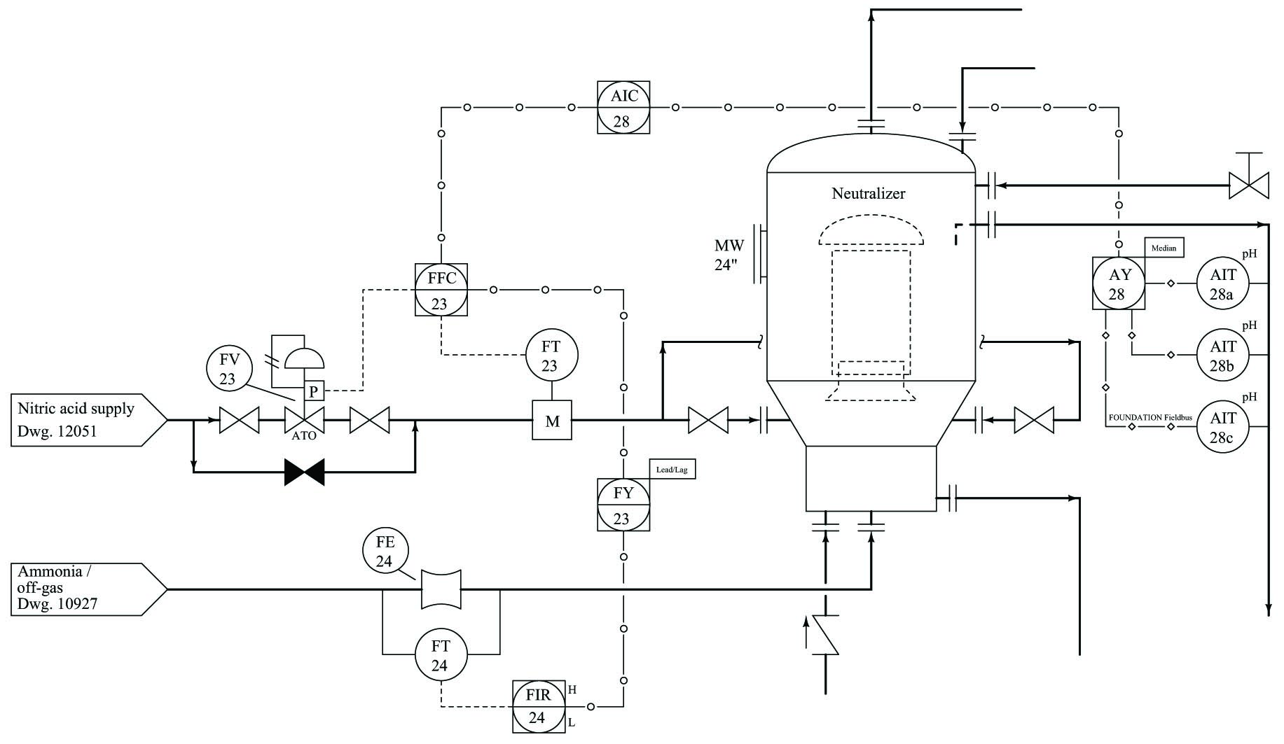
Before it is possible to analyze the effects of a transmitter failure, we must first determine what the system ought to do in normal operation. Natural questions to ask might include the following:
- Where do the instrument signals come from and where do they go to?
- What does each instrument signal represent?
- What is the direction of action for each controller in the system?
With just a basic understanding of ratio control systems, we may answer all of these questions by close examination of the P&ID segment, and also annotate those thoughts and conclusions on the diagram in order to help us analyze the system’s response. Starting with the first two questions of where signals originate and terminate and what each signal represents, we may annotate this with arrows and text (shown in red):
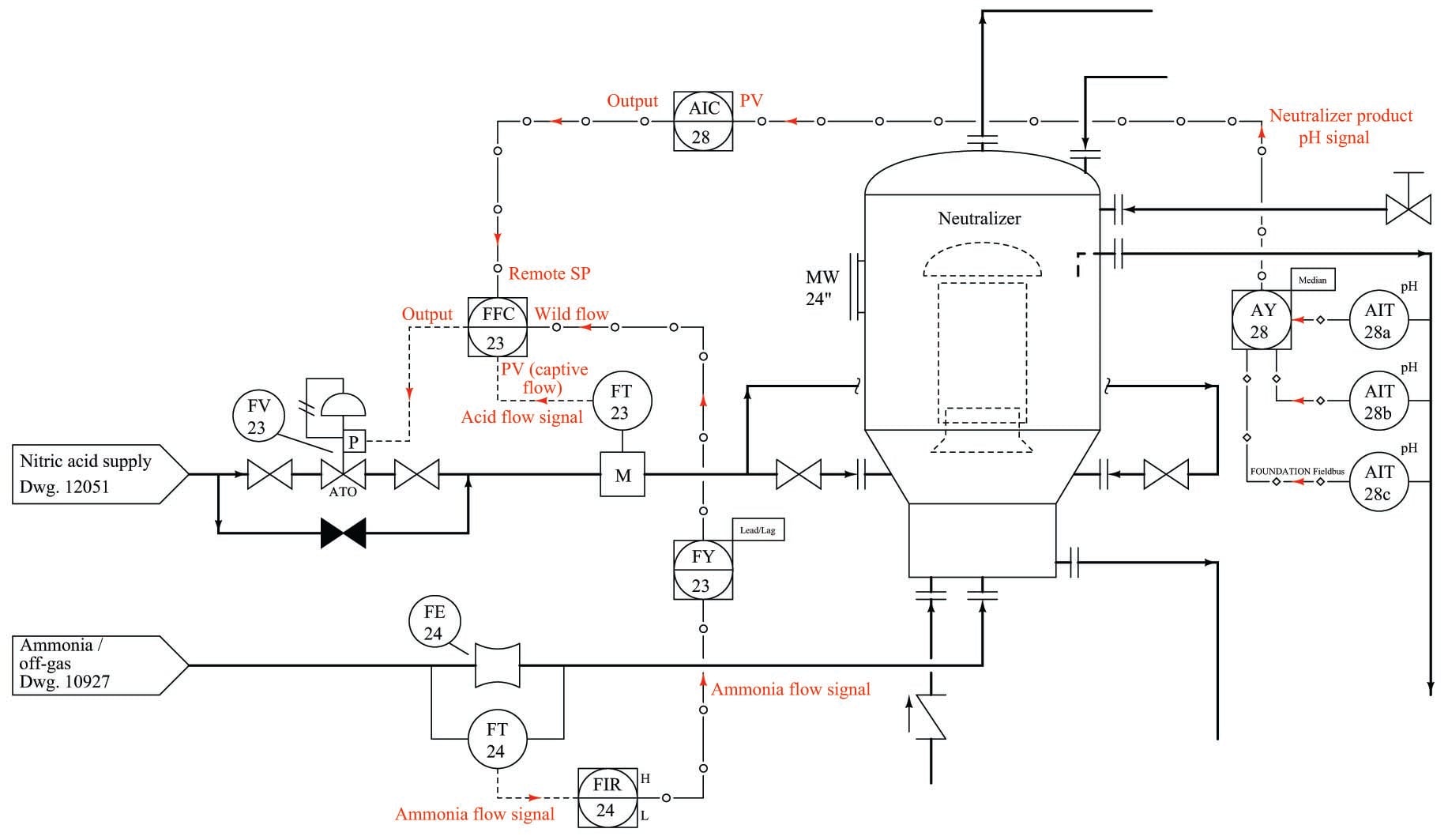
We know that all transmitters output data, and so all signal arrows should point away from all transmitters and toward all controllers. We know that all valves receive data, which means arrows must point toward the control valve. The first tag letter of each transmitter (AIT, FT) tells us its measurement function: chemical pH and flow, respectively. The fact that FT-23 is mounted on the same pipe as FV-23 tells us FT-23 must send controller FFC-23 its process variable (captive flow), making the other flow signal (from FT-24) the “wild” flow in this ratio control scheme. AIC-28’s task is to control pH exiting the neutralizer, so we know its output signal must call for a neutralizing reagent, in this case nitric acid. This tells us the signal between AIC-28 and FFC-23 must be a cascade output-setpoint link, with AIC-28 as the master controller and FFC-23 as the slave controller.
Now we turn to the question of controller action, since we know the direction of each controller’s action (e.g. direct or reverse) is significant to how each controller will react to any given change in signal. Here, ‘thought experiments’’ are useful as we imagine the process variable changing due to some load condition, and then determine how the controller must respond to bring that process variable back to setpoint.
When we annotate the action of each controller, it is best to use symbols more descriptive than the words “direct” and “reverse,” especially due to the confusion this often causes when distinguishing the effects of a changing PV signal versus a changing SP signal. In this case, we will write a short formula next to each controller denoting its action according to how the error is calculated (\(e = \hbox{PV} - \hbox{SP}\) for direct action and \(e = \hbox{SP} - \hbox{PV}\) for reverse action). We may also write “+” and “\(-\)” symbols next to each input on each controller to further reinforce the direction of each signal’s influence:
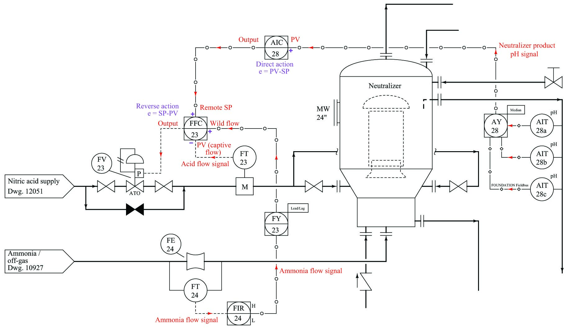
FFC-23 is the best controller to start with, since it is the slave controller (in the “inner-most” control loop of this cascade/ratio system). Here, we see that FFC-23 must be reverse-acting, for if FT-23 reports a higher flow we will want FV-23 to close down. This means the remote SP input must have a non-inverting effect on the output: a greater signal from AIC-28 will increase nitric acid flow into the neutralizer. Following this reasoning, we see that AIC-28 should be direct-acting, calling for more nitric acid flow into the neutralizer as product pH becomes more alkaline (pH increases).
The purpose of the ratio control strategy is to balance the “wild” flow of ammonia into the neutralizer with a proportional flow of nitric acid. This is in keeping with principles of chemical reactions (stoichiometry) and mass balance. Therefore, we would expect an increase in ammonia flow to call for a proportionate increase in nitric acid flow, giving the wild flow signal a non-inverting effect on FFC-23.
Only at this point in time are we fully ready to analyze the effects of FT-24 failing with a low-flow signal. Once again, we may annotate the failure on the diagram as well, arbitrarily electing to use blue “up” and “down” arrows and bold text to indicate the directions of change for each signal immediately following the failure of FT-24:
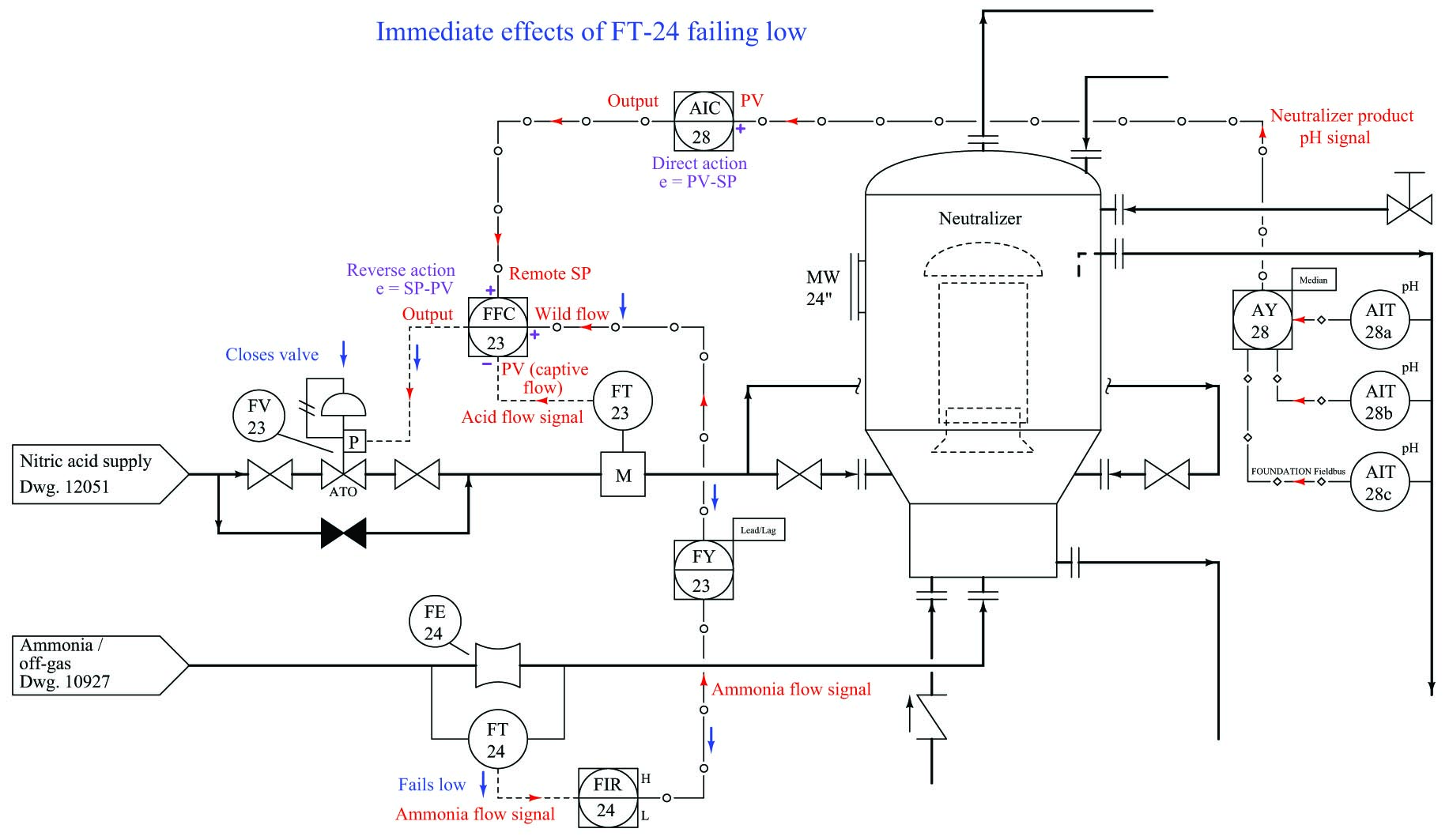
As FT-24’s signal fails low, the “wild” flow signal to FFC-23 goes low as well. Since we have already determined that input has a non-inverting effect on the ratio controller, we may conclude control valve FV-23 will close as a result, decreasing the flow of nitric acid into the neutralizer. This analysis becomes trivial after we’ve done the work of annotating the diagram with our own notes showing how the instruments are supposed to function. Without this set-up, the task of analyzing the effects of FT-24 failing low would be much more difficult.
