 Facebook
 Google
 GitHub
 Linkedin
Numerical Integration
As we have seen, the concept of integration is finding the accumulation of one variable multiplied by another (related) variable. In this section, we will explore the practical application of this concept to real-world data, where actual numerical values of variables are used to calculate accumulated sums.
In industrial instrumentation, for example, we are often interested in calculating the accumulation of some process fluid based on a measured flow rate of that fluid. The rate is, of course, expressed in either mass or volume units per unit time (e.g. gallons per minute), but the total accumulated quantity will be expressed plainly in either mass or volume units (e.g. gallons). We may use computers to calculate those accumulated quantities, either after the fact (from recorded data) or in real time.
Numerical (data-based) integration is fundamentally a two-step arithmetic process. First, we must use multiplication to calculate the product of a variable and a small increment of another variable (a change in the second variable between two different points). Then, we must use addition to calculate the accumulated sum of the products.
To illustrate, we will first focus on the integration of a flow measurement signal with respect to time. The flow rate of any fluid is always expressed in units of volume or mass per unit time. Common volumetric flow units are gallons per minute, liters per second, cubic feet per day, etc. Common mass flow units are pounds per hour, kilograms per minute, slugs per second, etc. If we desire to calculate the volume or mass of fluid passed through a pipe – representing fluid added to or removed from a system – over some interval of time, we may do so by integrating flow rate with respect to time:
\[\Delta V = \int_a^b Q \> dt\]
\[\Delta m = \int_a^b W \> dt\]
Where,
\(\Delta V\) = Volume of fluid added or removed
\(Q\) = Volumetric flow rate of fluid
\(\Delta m\) = Mass of fluid added or removed
\(W\) = Mass flow rate of fluid
\(a\) = Starting point of integration interval
\(b\) = Ending point of integration interval
\(t\) = Time
As always, integration is fundamentally a matter of multiplying one variable by small increments of another variable. If a flow rate is integrated with respect to time, the result is that the unit for time becomes eliminated. Gallons per minute, for example, becomes gallons after integration; kilograms per second becomes kilograms; etc.
The elimination of time units is also evident if we re-write the integrands in the previous equations to show volumetric and mass flow rates (\(Q\) and \(W\), respectively) as the rates of change they are (\(Q = {dV \over dt}\) and \(W = {dm \over dt}\)):
\[\Delta V = \int_a^b {dV \over dt} \> dt\]
\[\Delta m = \int_a^b {dm \over dt} \> dt\]
It should be clear that the time differentials (\(dt\)) cancel in each integrand, leaving:
\[\Delta V = \int_a^b dV\]
\[\Delta m = \int_a^b dm\]
Since we know the integral symbol (\(\int\)) simply means the “continuous sum of” whatever follows it, we may conclude in each case that the continuous sum of infinitesimal increments of a variable is simply a larger change of that same variable. The continuous summation of \(dV\) is simply the total change in \(V\) over the interval beginning at time \(a\) and ending at time \(b\); likewise, the continuous summation of \(dm\) is simply the total change in \(m\) over the interval beginning at time \(a\) and ending at time \(b\).
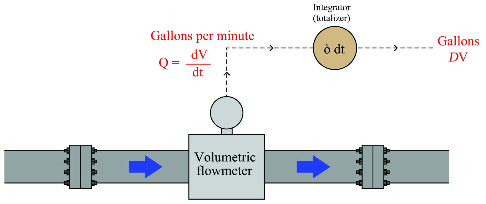
A flowmeter measuring the flow rate of a fluid outputs a signal representing either volume or mass units passing by per unit time. Integrating that signal with respect to time yields a value representing the total volume or mass passed through the pipe over a specific interval. A physical device designed to perform this task of integrating a signal with respect to time is called an integrator or a totalizer:
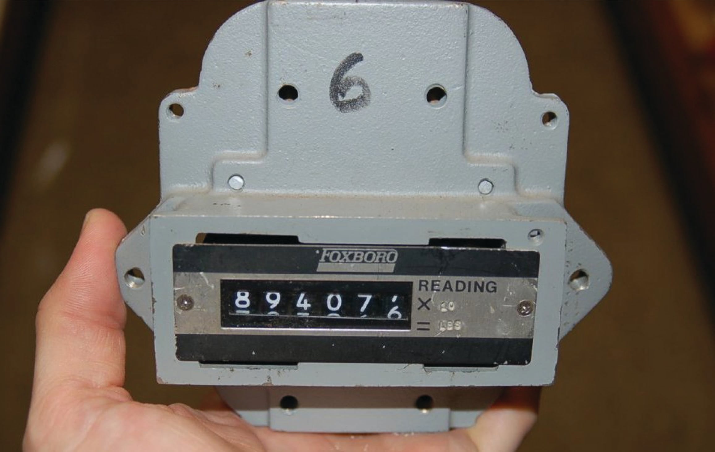
An example of a flow integrator, or flow totalizer, made for pneumatic instrument systems is the Foxboro model 14. A view of this instrument’s front face shows an odometer-style display, in this particular case showing the total number of pounds (lb) of fluid passed through the pipe, with a multiplying factor of 10:
The fact that this instrument’s display resembles the odometer of an automobile is no coincidence. Odometers are really just another form of mechanical integrator, “totalizing” the distance traveled by a vehicle. If the speedometer of a vehicle registers speed (\(v\)) in units of miles per hour, then the odometer will accumulate a distance (\(\Delta x\)) in units of miles, since distance (miles) is the time-integral of speed (miles per hour):
\[\Delta x = \int_a^b v \> dt \hskip 20pt \hbox{. . . or . . .} \hskip 20pt \Delta x = \int_a^b {dx \over dt} \> dt\]
\[[\hbox{miles}] = \int_a^b \left( \left[{\hbox{miles} \over \hbox{hour}}\right] \> [\hbox{hours}] \right)\]
In this particular case, where the flowmeter measures pounds per hour, and the integrator registers accumulated mass in pounds, the integration of units is as follows:
\[\Delta m = \int_a^b W \> dt \hskip 20pt \hbox{. . . or . . .} \hskip 20pt \Delta m = \int_a^b {dm \over dt} \> dt\]
\[[\hbox{pounds}] = \int_a^b \left( \left[{\hbox{pounds} \over \hbox{hour}}\right] \> [\hbox{hours}] \right)\]
The Foxboro model 14 used a turbine wheel driven by a jet of compressed air from a nozzle. The wheel’s speed was made proportional to the process fluid flow rate sensed by a pneumatic DP transmitter. As process flow rate increased, the wheel spun faster. This spinning wheel drove a gear-reduction mechanism to slowly turn the odometer-style numerals, registering total fluid quantity passed through the flowmeter:
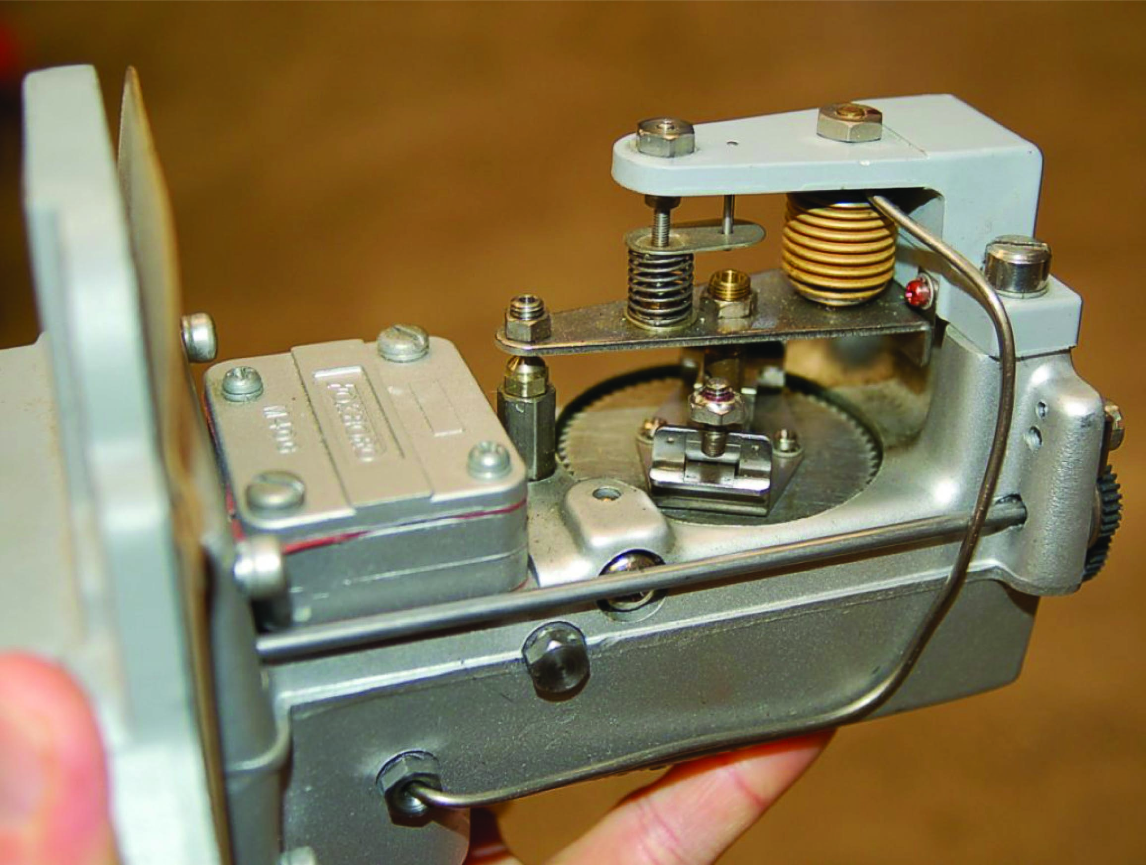
As pneumatic signal pressure (3-15 PSI) from a pneumatic flow transmitter entered the brass bellows of this instrument, it pressed down on a lever, forcing a baffle toward a nozzle. As nozzle backpressure rose, amplified air pressure spun the turbine wheel to drive the integrating “odometer” display. Mounted on the turbine wheel was a set of fly-weights, which under the influence of centrifugal force would press upward on the lever to re-establish a condition of force-balance to maintain a (relatively) constant baffle-nozzle gap. Thus, the force-balance mechanism worked to establish an accurate and repeatable relationship between instrument signal pressure and integration rate.
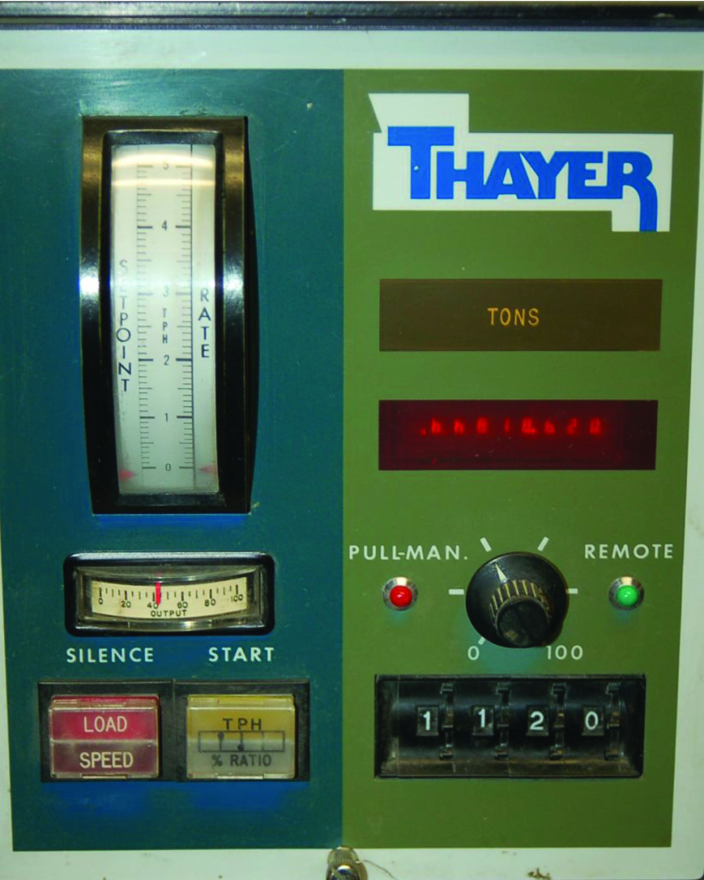
A very different style of integrator appears here, as part of the controller for a ball mill used to crush limestone into small pieces for the manufacturing of concrete. Limestone is fed into the ball mill on a device called a weighfeeder, which measures the mass of limestone as it passes over a conveyor belt. The controller maintains a limestone “flow rate” at a setpoint specified in tons per hour (mass flow of solid material). The red LED digital display shows the total number of tons passed through the mill:
The units involved in the integration of limestone “flow” into the ball mill are slightly different from the example shown with the Foxboro model 14 totalizer, but the concept is the same:
\[\Delta m = \int_a^b W \> dt\]
\[[\hbox{tons}] = \int_a^b \left( \left[{\hbox{tons} \over \hbox{hour}}\right] \> [\hbox{hours}] \right)\]
As with all cases of numerical integration, an essential piece of information to know when “totalizing” any rate is the initial quantity at the start of the totalization interval. This is the constant of integration mentioned previously. For flow totalization, this constant would be the initial volume of fluid recorded at the starting time. For an automobile’s odometer, this constant is the initial “mileage” accumulated prior to driving on a trip.
An algorithm applicable to integrating real signals with respect to time in a digital computer is shown here, once again using “pseudocode” as the computer language. Each line of text in this listing represents a command for the digital computer to follow, one by one, in order from top to bottom. The LOOP and ENDLOOP markers represent the boundaries of a program loop, where the same set of encapsulated commands are executed over and over again in cyclic fashion:
Pseudocode listing
LOOP
  SET x = analog_input_N      // Update x with the latest measured input
  SET t = system_time         // Sample the system clock

  SET delta_t = t - last_t    // Calculate change in t (time)

  SET product = x * delta_t   // Calculate product (integrand)
  SET total = total + product // Update the running total

  SET last_t = t              // Update last_t value for next program cycle
ENDLOOP
This computer program uses a variable to “remember” the value of time (\(t\)) from the previous scan, named last_t. This value is subtracted from the current value for \(t\) to yield a difference (delta_t), which is subsequently multiplied by the input value \(x\) to form a product. This product is then added to an accumulating total (named total), representing the integrated value. This “total” value may be sampled in some other portion of the computer’s program to trigger an alarm, a shutdown action, or simply display and/or record the totalized value for a human operator’s benefit.
The time period (\(\Delta t\)) for this program’s difference quotient calculation is simply how often this algorithm “loops,” or repeats itself. For a modern digital microprocessor, this could be upwards of many thousands of times per second. Unlike differentiation, where an excessive sampling rate may cause trouble by interpreting noise as extremely high rates of change, there is no danger of excessive sampling when performing numerical integration. The computer may integrate as fast as it can with no ill effect.
One of the fundamental characteristics of integration is that it ignores noise, which is a very good quality for industrial signal processing. Small “jittering” in the signal tends to be random, which means for every “up” spike of noise, one may expect a comparable “down” spike (or collection of “down” spikes having comparable weight) at some later time. Thus, noise tends to cancel itself out when integrated over time.
As with differentiation, applications exist for integration that are not time-based. One such application is the calculation of mechanical work, defined as the product of force and displacement (distance moved). In mechanical systems where there is no energy dissipated due to friction, work results in a change in the energy possessed by an object.
For example, if we use a hoist to lift a mass weighing 700 pounds straight up against gravity a distance of 3 feet, we will have done 2100 foot-pounds of work. The work done on the mass increases its potential energy (\(\Delta E\)) by 2100 foot-pounds:
\[\Delta E = Fx\]
Where,
\(\Delta E\) = Change in potential energy resulting from work, in joules (metric) or foot-pounds (British)
\(F\) = Force doing the work, in newtons (metric) or pounds (British)
\(x\) = Displacement over which the work was done, in meters (metric) or feet (British)
We may also express this change in potential energy as an integral of force (\(F\)) multiplied by infinitesimal increments in displacement (\(dx\)) over some interval (from \(a\) to \(b\)), since we know integration is nothing more than a sophisticated way to multiply quantities:
\[\Delta E = \int_a^b F \> dx\]
Like any other integral, the energy change effected by lifting this mass a vertical distance may be represented graphically as the area enclosed by the graph. In this case, the area is very simple to calculate, being a simple rectangle (height times width):
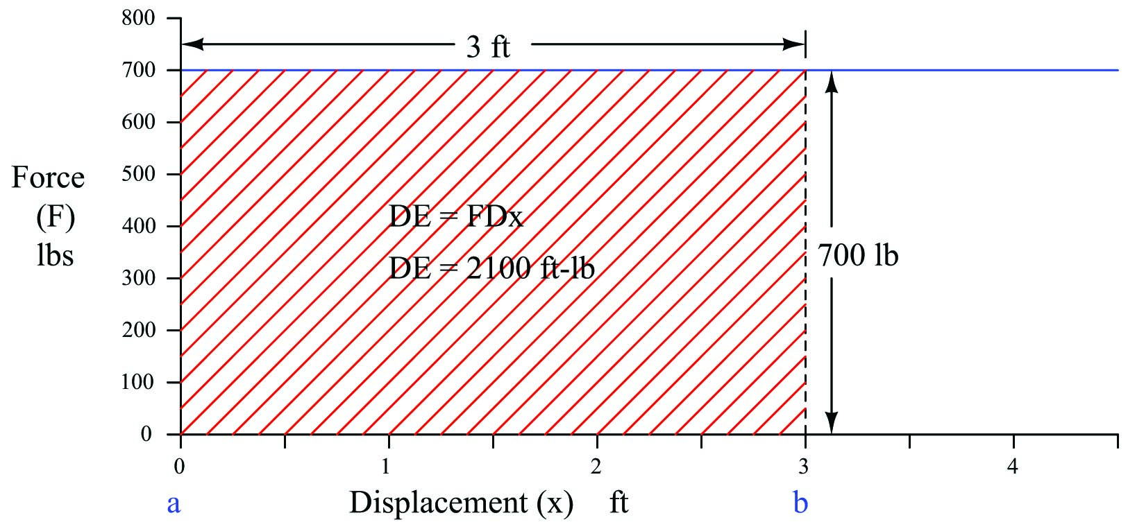
Lifting the mass vertically constitutes a positive change in potential energy for this object, because each displacement differential (\(dx\)) is a positive quantity as we move from a height of 0 feet to a height of 3 feet:
\[2100 \hbox{ ft-lbs} = \int_{0 ft}^{3 ft} (700 \hbox{ lbs}) \> dx\]
A natural question to ask at this point is, what would the resulting change in energy be if we the mass from its height of 3 feet back down to 0 feet?. Doing so would cover the exact same distance (3 feet) while exerting the exact same amount of suspending force (700 lbs), and so we can safely conclude the work will have an absolute magnitude of 2100 ft-lbs. However, if we lower the mass, each displacement differential (\(dx\)) will be a negative quantity22 as we move from a greater height to a lesser height. This makes the work – and the resulting energy change – a negative quantity as well:
\[-2100 \hbox{ ft-lbs} = \int_{3 ft}^{0 ft} (700 \hbox{ lbs}) \> dx\]
This means if we raise the mass to a height of 3 feet, then lower it back to its original starting height of 0 feet, the total change in potential energy will be zero:
\[0 \hbox{ ft-lbs} = \int_{0 ft}^{3 ft} (700 \hbox{ lbs}) \> dx + \int_{3 ft}^{0 ft} (700 \hbox{ lbs}) \> dx\]
This is true for any integral having an interval of zero (same starting and ending values), regardless of the integrand’s value at any point in time:
\[0 \hbox{ ft-lbs} = \int_a^a F \> dx\]
The integration of force and displacement to calculate potential energy change really shows its utility when the force changes as a function of displacement.
One practical example of this sort of calculation is the determination of energy stored in an archer’s bow when drawn to a certain displacement. The so-called force-draw curve of a longbow is nearly ideal for a theoretical spring, with force increasing linearly as the string is drawn back by the archer. The force-draw curve for a compound bow is quite nonlinear, with a much lesser holding force required to maintain the bow at full draw:
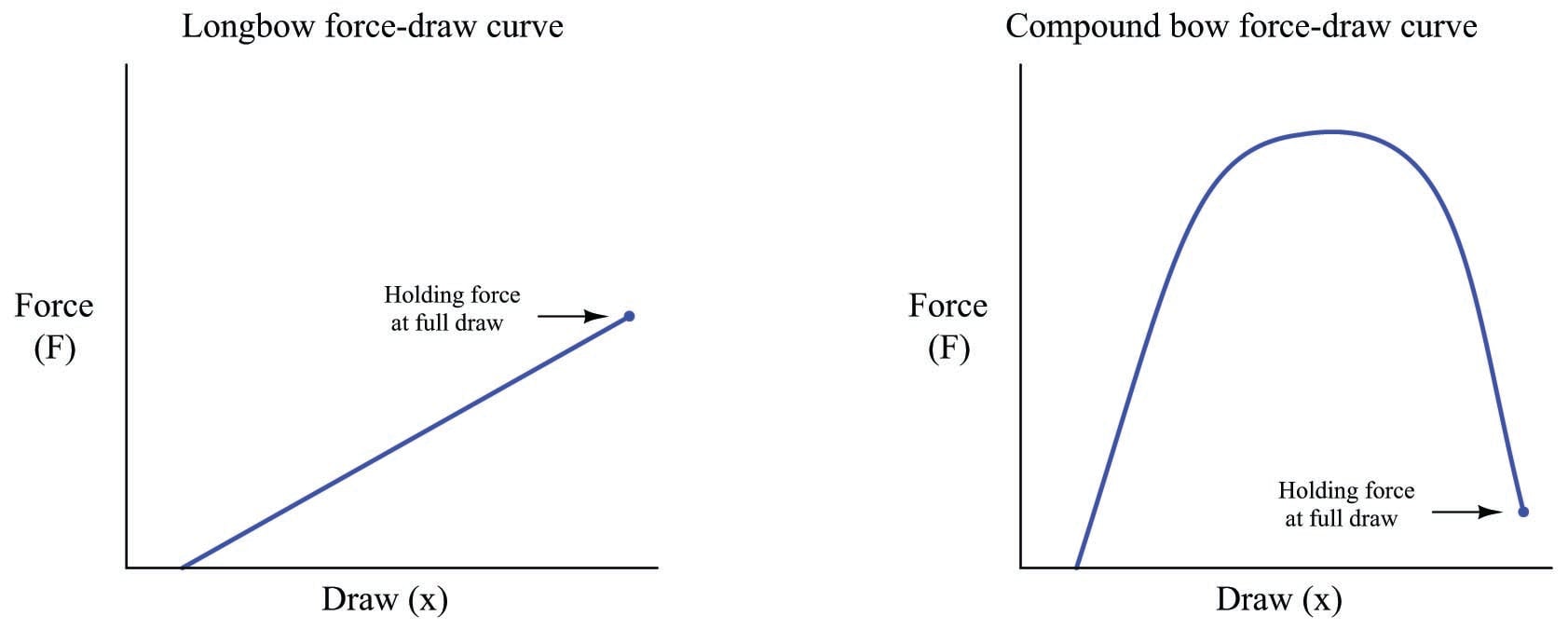
The force required to draw a compound bow rises sharply during the first few inches of draw, peaks during the region where the archer’s arms are ideally angled for maximum pulling strength, then “lets off” toward the end where the archer’s drawing arm is weakest in the “holding” position. The result is a bow that requires substantial force to draw, but is relatively easy to hold in fully-drawn position.
While the compound bow may be easier to hold at full draw than the longbow, for any given holding force the compound bow stores much more energy than the longbow, owing to the far greater area (force-displacement integral) enclosed by the curve:
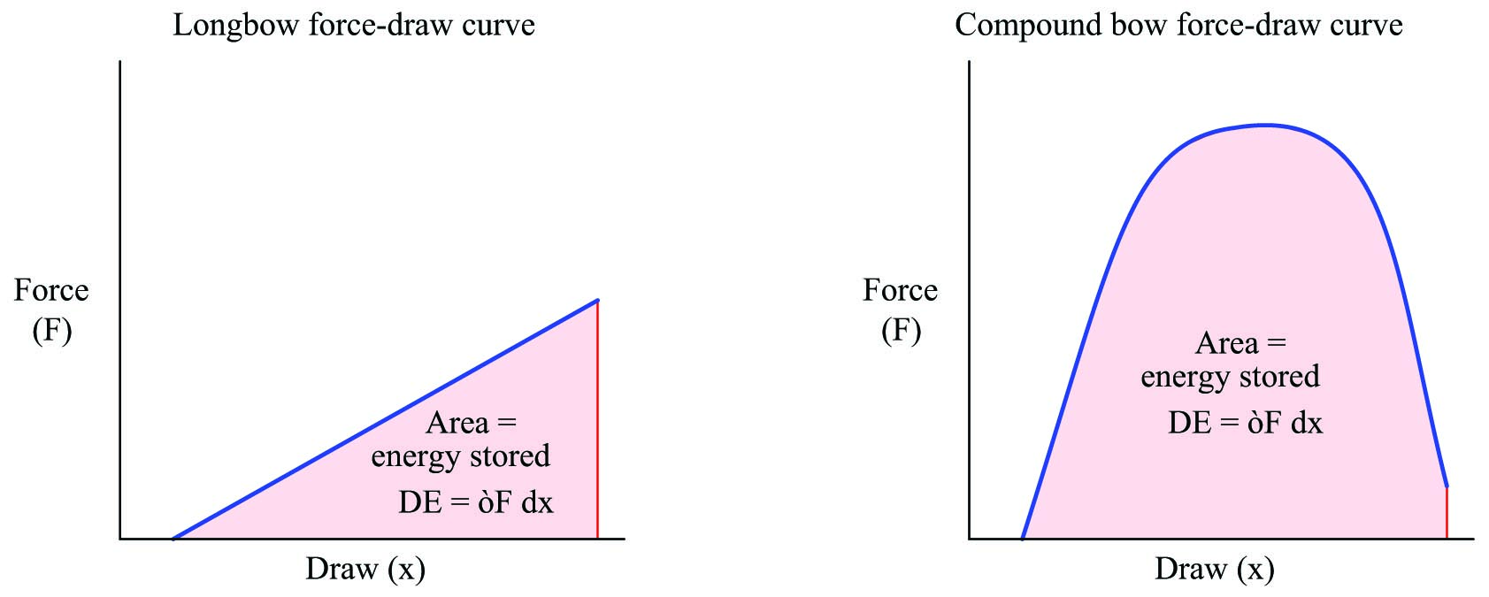
This is why a compound bow is so much more powerful than a longbow or a “recurve” bow with the same holding force: the energy represented by the greater area underneath the force-draw curve equates to greater energy imparted to the arrow when released, and therefore greater kinetic energy in the arrow during flight.
Like any other form of mechanical work, the energy invested into the bow by the archer is readily calculated and expressed in units of force \(\times\) displacement, typically newton-meters (joules) in metric units and foot-pounds in British units. This stands to reason, since we know integration is fundamentally a matter of multiplying quantities together, in this case force (pull) and displacement (draw).
To actually calculate the amount of energy stored in a fully-drawn bow, we could measure both force and displacement with sensors as the archer draws the bow, with a computer numerically integrating force over increments of draw in real time. Another method would be to simply graph force versus draw as we have done here, then use geometric methods24 to approximate the area underneath the curve.
A more sophisticated example of numerical integration used to calculate work is that of a heat engine, where a piston compresses an enclosed gas:
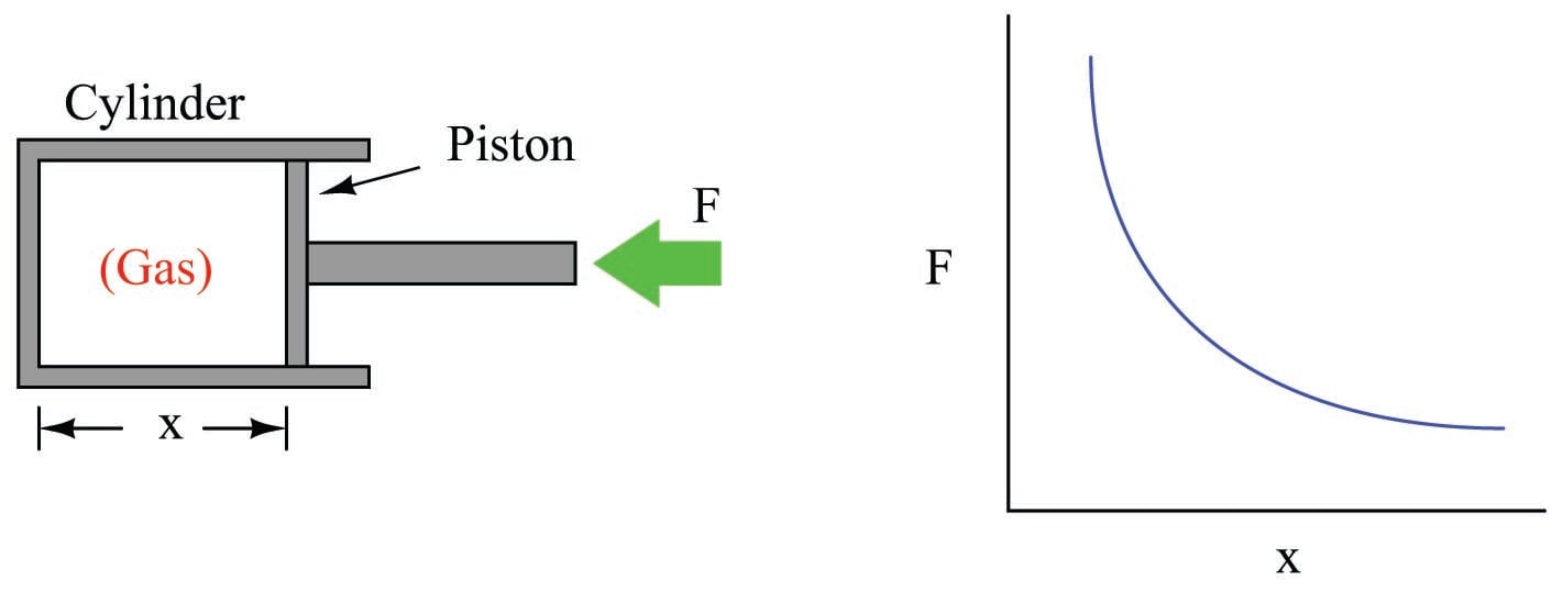
As the piston is pushed farther into the cylinder, the gas becomes compressed, exerting more force on the piston. This requires an ever-increasing application of force to continue the piston’s motion. Unlike the example where a mass of constant weight was lifted against the pull of gravity, here the force is a dynamically changing variable instead of a constant. The graph shows this relationship between piston displacement and piston force.
If we push the piston into the cylinder, the force increases as the displacement decreases. The change in energy is described by the integral of force with respect to displacement, graphically equivalent to the area underneath the force curve:
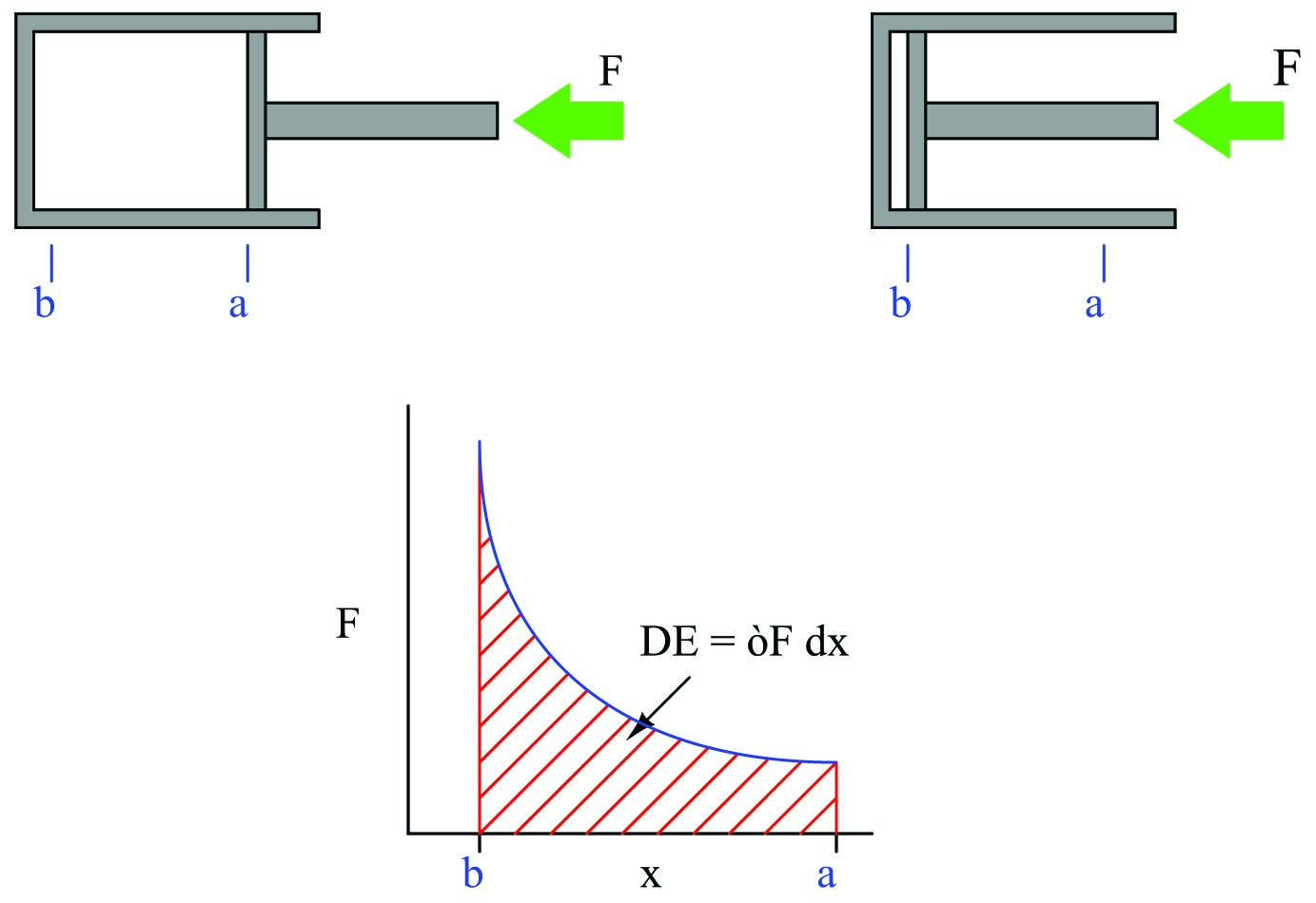
\[\Delta E = \int_a^b F \> dx\]
If we slowly allow the piston to return to its original position (letting the pressure of the enclosed gas push it back out), the piston’s force decreases as displacement increases. The force/displacement relationship is the same as before, the only difference being the direction of travel is opposite. This means the change in energy is happening over the same interval, in reverse direction (from \(b\) to \(a\) now instead of from \(a\) to \(b\)). Expressed as an integral:
\[\Delta E = \int_b^a F \> dx\]
As we have already learned, a reversal of direction means the sign of the integral will be opposite. If pushing the piston farther inside the cylinder represented work being done on the enclosed gas by the applied force, now the gas will be doing work on the source of the applied force as the piston returns to its extended position.
This means we will have done zero net work by pushing the piston into the cylinder and then letting it spring back out to its original position, just as we performed zero net work by lifting a mass 3 feet in the air and then letting it back down.
In order that this piston/cylinder mechanism might function as an engine, we must have some way of making the energy change greater in one direction than the other. This is done by heating the enclosed gas at the point of greatest compression. In a spark-ignition engine, the gas is actually a mixture of air and fuel, ignited by an electric spark. In a compression-ignition (diesel) engine, the gas is pure air, with fuel injected at the last moment to initiate combustion. The addition of heat (from combustion) will cause the gas pressure to rise, exerting more force on the piston than what it took to compress the gas when cold. This increased force will result in a greater energy change with the piston moving out of the cylinder than with the piston moving in:
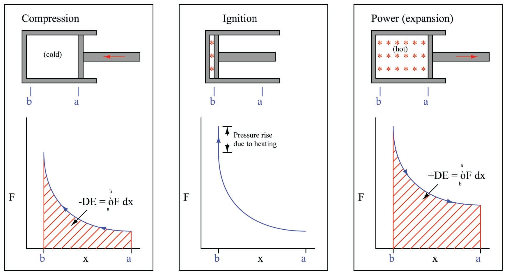
Representing the work done by the hot gas as the area enclosed by the curve makes this clear: more mechanical energy is being released as the piston travels from \(b\) to \(a\) during the “power stroke” than the amount of energy invested in compressing the gas as the piston traveled from \(a\) to \(b\) during the “compression stroke.” Thus, an internal combustion engine produces mechanical power by repeatedly compressing a cold gas, heating that gas to a greater temperature, and then expanding that hot gas to extract energy from it.
At the conclusion of the power stroke, a valve opens to exhaust the hot gas and another valve opens to introduce cold gas. This places the piston and cylinder in the original condition, ready for another set of compression, ignition, and power strokes. This cycle is sometimes represented as a closed “loop” on the force/displacement graph, like this:
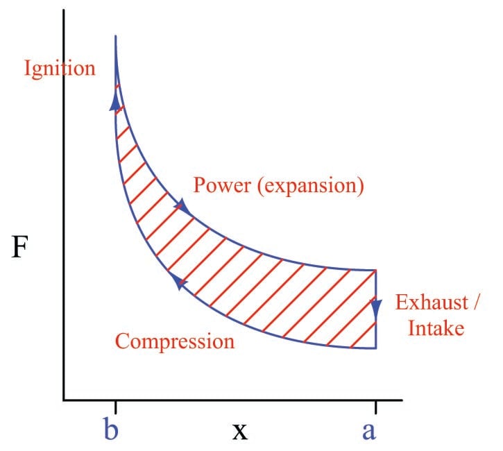
The amount of net energy output by the engine at the conclusion of each cycle is equivalent to the area enclosed by the loop. This is the difference in areas (integrals) between the “compression” and “power” strokes. Any design change to the engine resulting in a greater “loop” area (i.e. less energy required to compress the gas, and/or more energy extracted from its expansion) results in a more powerful engine. This is why heat engines output the most power when the difference in temperatures (cold gas versus heated gas) is greatest: a greater temperature shift results in the two curves being farther apart vertically, thus increasing the area enclosed by the “loop.”
