 Facebook
 Google
 GitHub
 Linkedin
Problem-solving by Simplification
A whole class of problem-solving techniques focuses on altering the given problem into a simpler form that is easier to analyze. Once a solution is found to the simplified problem, fresh ideas for attacking the original problem often become clear. This section will highlight multiple techniques for problem-simplification, as well as other useful techniques for problem-solving.
The first step, however, to problem simplification is to “give yourself the right” to alter the problem into a different form! Many students tend to avoid this, for fear of “getting off track” and losing sight of the original problem. What is needed is a spirit of adventure: a willingness and a confidence to explore the possibilities. Do not think you must solve exactly the problem that is given to you at first. Modify the problem, solve the simpler version of that problem, then apply the lessons and patterns obtained from that solution to the original (more complex) problem!
Limiting cases
A powerful method for analyzing the effects of a change in some system is to consider the effects of “extreme” changes, which are often easier to visualize than subtle changes. Such “extreme” changes are examples of what is generally known in science as a limiting case: a special case of a more general rule or trend, possessing fewer possibilities. By virtue of the fact that limiting cases have fewer possibilities, applying a limiting case to a given problem generally simplifies that problem.
Consider, for example, this Wheatstone bridge circuit, where changes in the thermistor’s resistance (with temperature) affect the output voltage of the bridge:
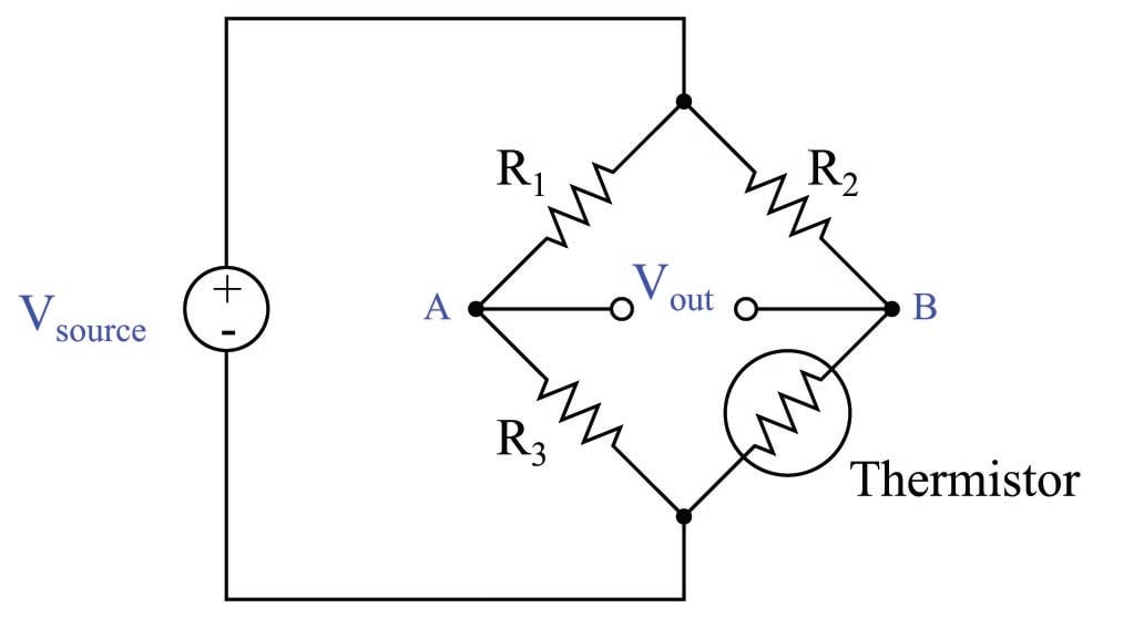
A realistic question to ask of this circuit is, “what will happen to \(V_{out}\) when the thermistor’s resistance increases?” If our only goal is to arrive at a qualitative answer (e.g. increase/decrease, positive/negative), we may simplify the problem by considering the effects of the thermistor failing completely open, because an “open” fault is nothing more than an extreme example (a limiting case) of a resistance increase.
If we perform this “thought experiment” on the bridge circuit, the circuit becomes simpler because we have eliminated one resistor (the thermistor):
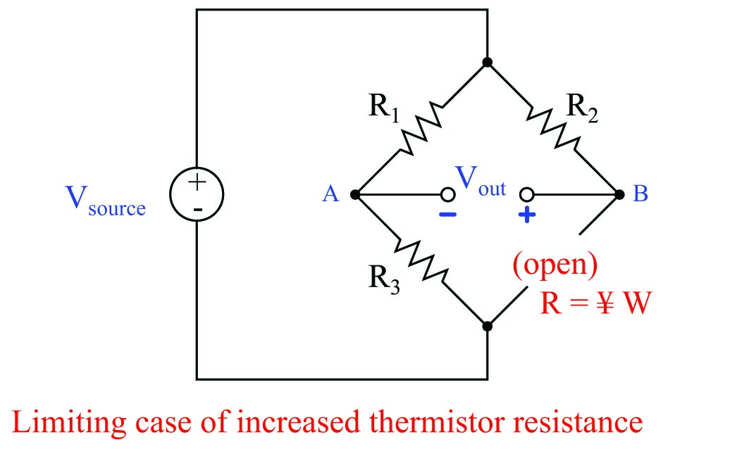
With the thermistor eliminated from the circuit, we see that test point B has lost its connection to the negative terminal of the voltage source. This can only mean one thing for the potential at test point B: it will become more positive (less negative). If the bridge circuit happened to be balanced prior to the thermistor fault, \(V_{out}\) will now be such that B is positive and A is negative by comparison.
Analyzing the results of this limiting case even further, we can see that resistor \(R_2\) now carries zero current (thanks to the thermistor now being failed open), which means \(R_2\) will now drop zero voltage. If \(R_2\) drops no voltage at all, test point B must now be at the exact same potential as the positive terminal of the voltage source. This being the case, measuring \(V_{out}\) between test points A and B will be equivalent to measuring voltage across \(R_1\). Thus, the limiting case of \(V_{out}\) for an increase in thermistor resistance is \(V_{R1}\), with B positive and A negative.
Another realistic question to ask of this circuit is, “what will happen to \(V_{out}\) when the thermistor’s resistance decreases?” Once again, the problem-solving technique of limiting cases helps us by transforming the four-resistor bridge circuit into a three-resistor bridge circuit. The limiting case of a resistance decrease would be a condition of no resistance: a shorted thermistor:
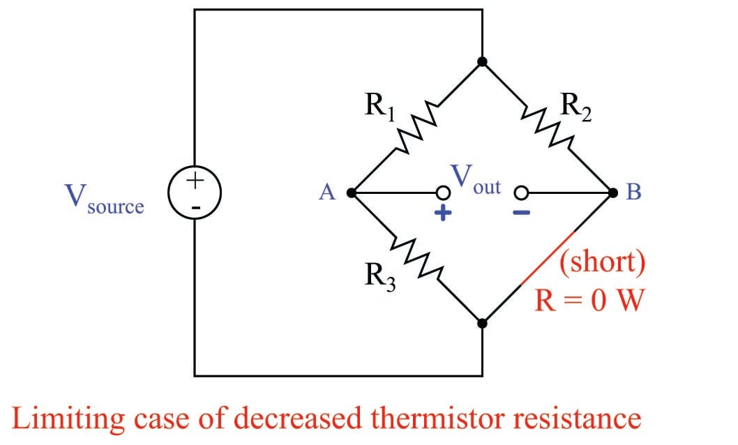
With the thermistor shorted in this “thought experiment,” we see that test point B now becomes electrically common with the negative terminal of the voltage source. This, of course, has the effect of making test point B as negative as it can possibly be. More specifically, by making test point B electrically common with the bottom node of the bridge, it makes \(V_{out}\) equal to the voltage drop across \(R_3\). Thus, the limiting case of \(V_{out}\) for a decrease in thermistor resistance is \(V_{R3}\), with A positive and B negative.
Let us consider another application of this problem-solving technique, this time to the analysis of a passive filter circuit:
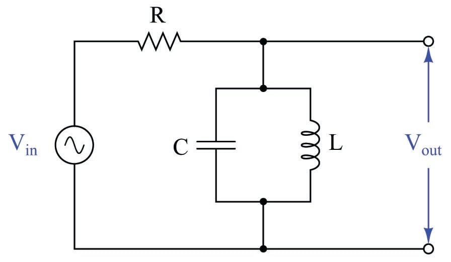
If the type of filter circuit shown here were unknown (i.e. the student could not identify it as a low-pass, high-pass, band-pass, or band-stop filter circuit at first sight), the technique of limiting cases could be applied to determine its behavior. In this case, the limit to apply is one of frequency: we may perform “thought experiments” whereby we imagine the input frequency being extremely low, versus being extremely high.
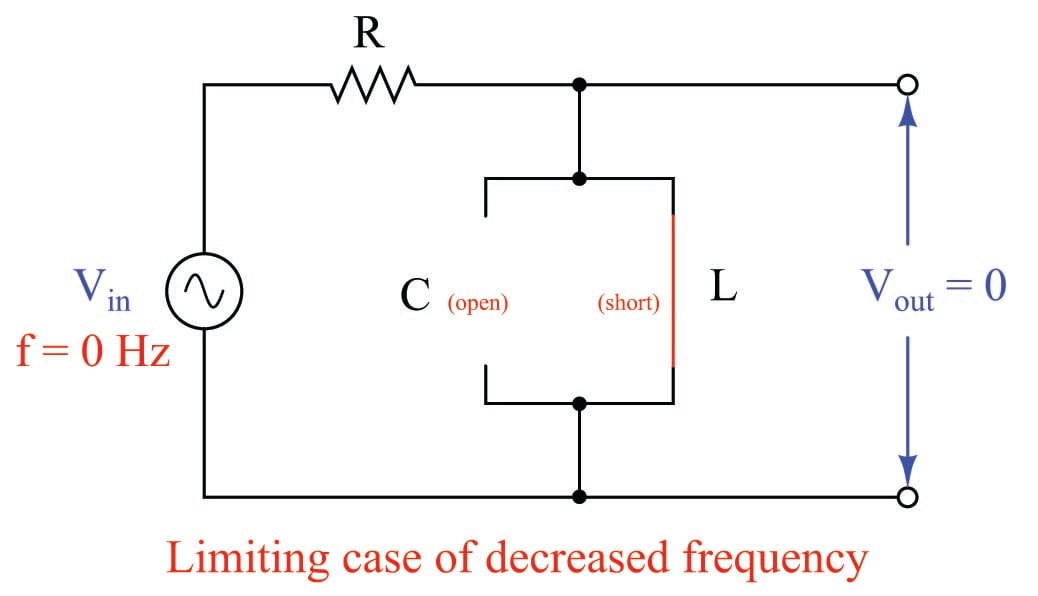
We know that the reactance of an inductor is directly proportional to frequency (\(X_L = 2 \pi f L\)) and that the reactance of a capacitor is inversely proportional to frequency (\(X_C = {1 \over {2 \pi f C}}\)). Therefore, at an extremely low frequency (\(f =\) 0 Hz), the inductor will act like a short while the capacitor acts like an open:
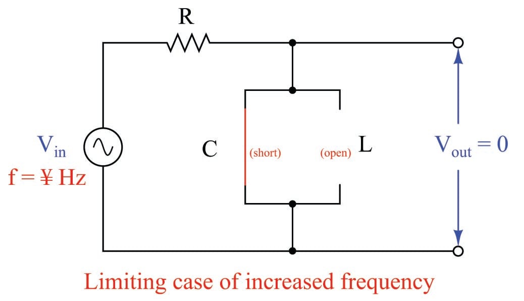
Likewise, at extremely high frequencies (\(f = \infty\)), the capacitor will act like a short while the inductor acts like an open:
From these two limiting-case “thought experiments” we may conclude that the filter circuit is neither a low-pass nor a high-pass, because it neither passes low-frequency signals nor high-frequency signals. We may also conclude that it is not a band-stop filter, because that would pass both low-frequency and high-frequency signals. This means it must be a band-pass filter, by eliminating the other three alternatives.
If we would wish to confirm the band-pass nature of this filter by a positive experimental result rather than merely by eliminating what it is not, we could perform one more limiting-case “thought experiment:” a condition where the signal frequency exactly equals the resonant frequency of the LC network (\(f = {1 \over 2 \pi \sqrt{LC}}\)). Here, we must recall the principle that a parallel LC network has infinite impedance at its resonant frequency:
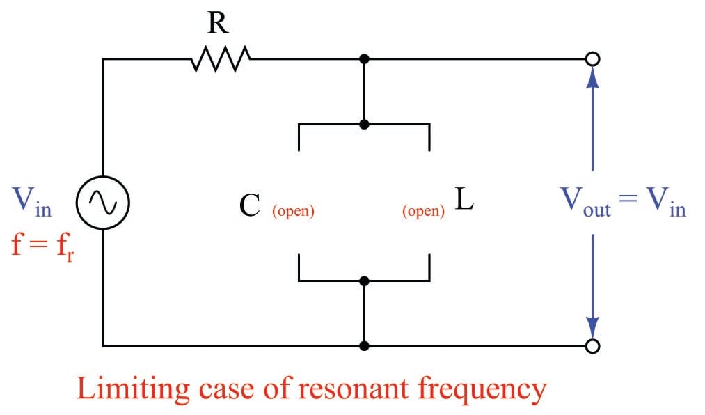
In this “thought experiment” we see that the LC network will be completely “open” and allow 100% of the input signal to appear at the output terminals. Thus, it becomes clear that this passive circuit functions as a band-pass filter.
As with the Wheatstone bridge circuit, the value of limiting-case analysis is that it acts to simplify the system by effectively eliminating components (replacing them with “shorts” or “opens”). Even in non-electrical problems, limiting cases works the same by simplifying a system’s behavior so that it becomes easier to apprehend, and from these simplified cases we may usually determine behavioral trends of the system (e.g. which way it tends to respond as some variable increases or decreases).
