 Facebook
 Google
 GitHub
 Linkedin
Root Mean Square (RMS) Quantities
Why can't we measure AC and DC voltage the same way?
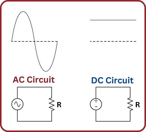
Root mean square, or RMS, is the DC equivalent output value of a sine wave, like an AC waveform. Since AC alternates polarities, but power output does not, expressing AC as a positive equivalent is very important.
It is often useful to express the amplitude of an alternating quantity such as voltage or current in terms that are equivalent to direct current (DC). Doing so provides an “apples-to-apples” comparison between AC and DC quantities that makes comparative circuit analysis much easier.
RMS Value of an AC Waveform
The most popular standard of equivalence is based on work and power, and we call this the root-mean-square value of an AC waveform, or RMS for short. For example, an AC voltage of 120 volts “RMS” means that this AC voltage is capable of delivering the exact same amount of power (in Watts) at an electrical load as a 120 volt DC source powering the exact same load.
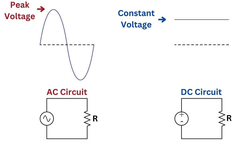
The problem is exactly how to calculate this “RMS” value if all we know about the AC waveform is its peak value. If we compare a sine wave and a DC “wave” side by side, it is clear that the sine wave must peak at a greater value than the constant DC level in order to be equivalent in terms of doing the same work in the same amount of time:
At first, it might seem like the correct approach would be to use calculus to integrate (determine the area enclosed by) the sine wave over one-half of a cycle: from 0 to \(\pi\) radians. This is close, but not fully correct. The ability of an electrical voltage to dissipate power at a resistor is not directly proportional to the magnitude of that voltage, but rather proportional to the square of the magnitude of that voltage! In mathematical terms, resistive power dissipation is predicted by the following equation:
\[P = {V^2 \over R}\]
If we double the amount of voltage applied to a resistor, the power increases four-fold. If we triple the voltage, the power goes up by a factor of nine. If we are to calculate the “RMS” equivalent value of a sine wave, we must take this nonlinearity into consideration.
Work and Power in a DC Circuit
First let us begin with a mathematical equivalence between the DC and AC cases. For DC, the amount of work done is equal to the constant power of that circuit multiplied by time. The unit of measurement for power is the Watt, which is defined as 1 Joule of work per second. So, multiplying the steady power rate in a DC circuit by the time we keep it powered will result in an answer of joules (total energy dissipated by the resistor):
\[\hbox{Work} = \left({V^2 \over R} \right)t\]
Showing this equivalence by dimensional analysis:
\[[\hbox{Joules}] = \left([\hbox{Joules}] \over [\hbox{s}]\right) [\hbox{s}]\]
Work and Power in an AC Circuit
We cannot calculate the work done by the AC voltage source quite so easily, because the power dissipation varies over time as the instantaneous voltage rises and falls. Work is still the product of power and time, but we cannot simply multiply one by the other because the voltage in this case is a function of time (\(V(t)\)). Instead, we must use integration to calculate the product of power and time, and sum those work quantities into a total work value.
Since we know the voltage provided by the AC source takes the form of a sine wave (\(V(t) = \sin t\) if we assume a sine wave with a peak value of 1 volt), we may write the formula for instantaneous AC power as follows:
\[\hbox{Power} = {\left(V(t)\right)^2 \over R} = {\sin^2 t \over R}\]
To calculate the work done by this sinusoidal voltage on the resistor, we will integrate this instantaneous power with respect to time, between the intervals of \(t=0\) and \(t=\pi\) (one half-cycle of the sine wave):
\[\hbox{Work} = \int_0^\pi {{\sin^2 t} \over R} \> dt\]
In order to solve for the amount of DC voltage equivalent (from the perspective of resistive power dissipation) to a one-volt AC sine wave, we will set the DC work and AC work equations equal to each other, making sure the DC side of the equation has \(\pi\) for the amount of time (being the same time interval as the AC side):
\[\left({V^2 \over R} \right) \pi = \int_0^\pi {{\sin^2 t} \over R} \> dt\]
Our goal is to solve for \(V\) on the left-hand side of this equation.
First, we know that \(R\) is a constant value, and so we may move it out of the integrand:
\[\left({V^2 \over R} \right) \pi = {1 \over R} \int_0^\pi \sin^2 t \> dt\]
Multiplying both sides of the equation by \(R\) eliminates it completely. This should make intuitive sense, as our RMS equivalent value for an AC voltage is defined strictly by the ability to produce the same amount of power as the same value of DC voltage for any resistance value. Therefore the actual value of resistance (\(R\)) should not matter, and it should come as no surprise that it cancels:
\[V^2 \pi = \int_0^\pi \sin^2 t \> dt\]
Now, we may simplify the integrand by substituting the half-angle equivalence for the \(\sin^2 t\) function
\[V^2 \pi = \int_0^\pi {{1 - \cos 2t} \over 2} \> dt\]
Factoring one-half out of the integrand and moving it outside (because it’s a constant):
\[V^2 \pi = {1 \over 2}\int_0^\pi 1 - \cos 2t \> dt\]
We may write this as the difference between two integrals, treating each term in the integrand as its own integration problem:
\[V^2 \pi = {1 \over 2} \left( \int_0^\pi 1 \> dt - \int_0^\pi \cos 2t \> dt \right)\]
The second integral may be solved simply by using substitution, with \(u = 2t\), \(du = 2 \> dt\), and \(dt = {du \over 2}\):
\[V^2 \pi = {1 \over 2} \left( \int_0^\pi 1 \> dt - \int_0^\pi {\cos u \over 2} \> du \right)\]
Moving the one-half outside the second integrand:
\[V^2 \pi = {1 \over 2} \left( \int_0^\pi 1 \> dt - {1 \over 2}\int_0^\pi \cos u \> du \right)\]
Finally we are at a point where we may perform the integrations:
\[V^2 \pi = {1 \over 2} \left( \int_0^\pi 1 \> dt - {1 \over 2}\int_0^\pi \cos u \> du \right)\]
\[V^2 \pi = {1 \over 2} \left( \left[ t \right]_0^\pi - {1 \over 2}\left[\sin 2t \right]_0^\pi \right)\]
\[V^2 \pi = {1 \over 2} \left( [\pi - 0] - {1 \over 2}[\sin 2\pi - \sin 0] \right)\]
\[V^2 \pi = {1 \over 2} \left( [\pi - 0] - {1 \over 2}[0 - 0] \right)\]
\[V^2 \pi = {1 \over 2} (\pi - 0)\]
\[V^2 \pi = {1 \over 2}\pi\]
We can see that \(\pi\) cancels out of both sides:
\[V^2 = {1 \over 2}\]
Taking the square root of both sides, we arrive at our final answer for the equivalent DC voltage value:
\[V = {1 \over \sqrt{2}}\]
So, for a sinusoidal voltage with a peak value of 1 volt, the DC equivalent or “RMS” voltage value would be \({1 \over \sqrt{2}}\) volts, or approximately 0.707 volts. In other words, a sinusoidal voltage of 1 volt peak will produce just as much power dissipation at a resistor as a steady DC voltage of 0.7071 volts applied to that same resistor. Therefore, this 1 volt peak sine wave may be properly called a 0.7071 volt RMS sine wave, or a 0.7071 volt “DC equivalent” sine wave.
This factor for sinusoidal voltages is quite useful in electrical power system calculations, where the wave-shape of the voltage is nearly always sinusoidal (or very close). In your home, for example, the voltage available at any wall receptacle is 120 volts RMS, which translates to 169.7 volts peak.
Electricians and electronics technicians often memorize the \(1 \over \sqrt{2}\) conversion factor without realizing it only applies to sinusoidal voltage and current waveforms. If we are dealing with a non-sinusoidal wave-shape, the conversion factor between peak and RMS will be different! The mathematical procedure for obtaining the conversion factor will be identical, though: integrate the wave-shape’s function (squared) over an interval sufficiently long to capture the essence of the shape, and set that equal to \(V^2\) times that same interval span.
REVIEW:
-
AC waveforms require a DC equivalent to represent the actual work done. This is the root mean square, or RMS value.
-
The relationship of 0.7071 is the ratio between peak value:RMS value. The RMS value will always be lower than peak.
-
RMS values only apply to sine waves. Any other alternating wave, such as audio, must be integrated, but only if a consistent signal can be identified.
