 Facebook
 Google
 GitHub
 Linkedin
Phasors, Phase Shift, and Phasor Algebra
The alternating nature of AC waves requires a way to express varying degrees of positive and negative polarity
The combinations of capacitors, inductors, and resistors in AC circuits work together to create shifts in the timing of voltage and current waves. Phasors define this relationship between voltage, reactance, impedance, and current.
Phasors are to AC circuit quantities as polarity is to DC circuit quantities: a way to express the “directions” of voltage and current waveforms. As such, it is difficult to analyze AC circuits in depth without using this form of mathematical expression. Phasors are based on the concept of complex numbers: combinations of “real” and “imaginary” quantities. The purpose of this section is to explore how complex numbers relate to sinusoidal waveforms, and show some of the mathematical symmetry and beauty of this approach.
Since waveforms are not limited to alternating current electrical circuits, phasors have applications reaching far beyond the scope of this chapter.
Circles, Sine Waves, and Cosine Waves
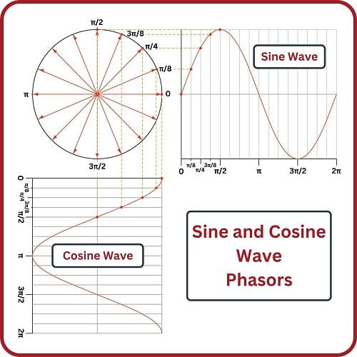
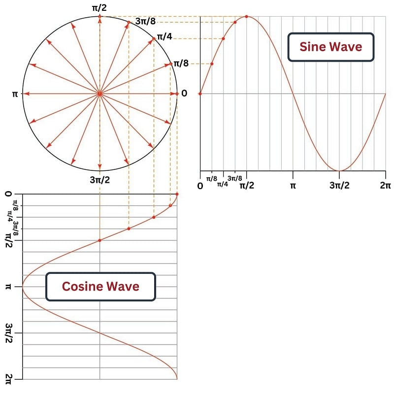
Something every beginning trigonometry student learns (or should learn) is how sine and cosine waves may be derived from a circle. First, sketch a circle, then sketch a set of radius vectors from the circle’s center to the circle’s perimeter at regular angle intervals. Mark each point of intersection between a vector and the circle’s perimeter with a dot and label each with the vector angle. Sketch rectangular graphs to the right and below the circle, with regularly-spaced divisions. Label those divisions with the same angles as the vectors and then sketch dashed “projection” lines from each vector tip to the respective divisions on the rectangular graphs, marking each intersection with a dot. Connect the dots with curves to reveal sinusoidal waveshapes.
The following illustration shows the dots and projection lines for the first five vectors (angles 0 through \(\pi \over 2\) radians) only. As you can see, the circle’s vertical projection forms a sine wave, while the circle’s horizontal projection forms a cosine wave:

Euler's Relation
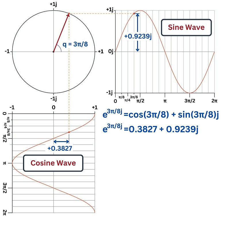
The Swiss mathematician Leonhard Euler (1707-1783) developed a symbolic equivalence between polar (circular) plots, sine waves, and cosine waves by plotting the circle on a complex plane where the vertical axis is an “imaginary” number line and the horizontal axis is a “real” number line. Euler’s Relation expresses the vertical (imaginary) and horizontal (real) projections of an imaginary exponential function as a complex (real + imaginary) trigonometric function:
\[e^{j \theta} = \cos \theta + j \sin \theta\]
Where,
\(e\) = Euler’s number (approximately equal to 2.718281828)
\(\theta\) = Angle of vector, in radians
\(\cos \theta\) = Horizontal projection of a unit vector (along a real number line) at angle \(\theta\)
\(j\) = Imaginary “operator” equal to \(\sqrt{-1}\), represented by \(i\) or \(j\)
\(j \sin \theta\) = Vertical projection of a unit vector (along an imaginary number line) at angle \(\theta\)
To illustrate, we will apply Euler’s relation to a unit vector having an angular displacement of \(3 \pi \over 8\) radians:
This mathematical translation from circles to sinusoidal waves finds practical application in AC electrical systems, because the rotating vector directly relates to the rotating magnetic field of an AC generator while the sinusoidal function directly relates to the voltage generated by the field’s motion. The principle of an AC generator is that a magnet rotates on a shaft past stationary coils of wire. When these wire coils experience the changing magnetic field produced by the rotating magnet, a sinusoidal voltage is induced:
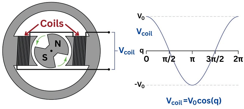
If we mark the shaft of this simple two-pole generator such that an angle of zero is defined as the position where the stator coils develop maximum positive voltage (\(V_0\)), the AC voltage waveform will follow the cosine function as shown above. If we were to add another set of stationary (“stator”) coils to the generator’s frame perpendicular to this set, that second set of coils would generate an AC voltage following the sine function. As it is, there is no second set of stator coils, and so this sine-function voltage is purely an imaginary quantity whereas the cosine-function voltage is the only “real” electricity output by the generator.
The canonical form of Euler’s Relation assumes a circle with a radius of 1. In order to realistically represent the output voltage of a generator, we may include a multiplying coefficient in Euler’s Relation representing the function’s peak value:
\[Ae^{j \theta} = A \cos \theta + j A \sin \theta\]
In the case of the generator shown above, the \(A\) coefficient is the peak voltage (\(V_0\)) output by the stator coils at the precise moment in time when the shaft angle is zero. In other words, the exponential term (\(e^{j \theta}\)) tells us which way the vector points while the coefficient (\(A\)) tells us how long the vector is.
In electrical studies it is commonplace to use various “shorthand” notations for vectors. An instantaneous quantity (e.g. voltage or current at some moment in time) described simply in terms of real and imaginary values is called rectangular form, for example 0.3827 + \(j\)0.9239 volts. An instantaneous quantity described simply in terms of vector angle and length is called polar form, for example 1 volt \(\angle\) 67.5\(^{o}\). Euler’s Relation is the mathematical link connecting rectangular and polar forms.
| Polar | Rectangular | |
|---|---|---|
| Shorthand notation | \(A \angle \theta\) | \(x + jy\) |
| Full notation | \(Ae^{j \theta}\) | \(A \cos \theta + j A \sin \theta\) |
All of these vectors described by the imaginary exponential function \(e^{j \theta}\) are of a special kind – vectors inhabiting a space defined by one real axis and one imaginary axis (the so-called complex plane). In order to avoid confusing this special quantity with real vectors used to represent quantities in actual space where every axis is real, we use the term phasor instead. From this point on in the book, I will use the term “phasor” to describe complex quantities as represented in Euler’s Relation, and “vector” to describe any other quantity possessing both a magnitude and a direction.
Euler’s Relation may also be used to describe the behavior of the rotating generator shaft and its corresponding AC voltage output as a function of time. Instead of specifying a shaft position (angle \(\theta\)) we now specify a point in time (\(t\)) and an angular velocity (rotational speed) represented by the lower-case Greek letter “omega” (\(\omega\)). Since angular velocity is customarily given in units of radians per second, and time is customarily specified in seconds, the product of those two will be an angle in radians (\(\omega t = \theta\)). Substituting \(\omega t\) for \(\theta\) in Euler’s Relation gives us a function describing the state of the generator’s output voltage in terms of time:
\[Ae^{j \omega t} = A \cos \omega t + j A \sin \omega t\]
Where,
\(A\) = Peak amplitude of generator voltage, in volts
\(e\) = Euler’s number (approximately equal to 2.718281828)
\(\omega\) = Angular velocity, in radians per second
\(t\) = Time, in seconds
\(\cos \omega t\) = Horizontal projection of phasor (along a real number line) at time \(t\)
\(j\) = Imaginary “operator” equal to \(\sqrt{-1}\), represented by \(i\) or \(j\)
\(j \sin \omega t\) = Vertical projection of phasor (along an imaginary number line) at time \(t\)
With just a little bit of imagination we may visualize both the exponential and complex sides of Euler’s Relation in physical form. The exponential (\(e^{j \omega t}\)) is a phasor rotating counter-clockwise about a central point over time. The complex (\(\cos \omega t + j \sin \omega t\)) is a pair of cosine and sine waves oscillating along an axis of time. Both of these manifestations may be joined into one visual image if you imagine a corkscrew where the centerline of the corkscrew is the time axis, and the evolution of this function over time follows the curve of the corkscrew down its length. Viewed from one end (looking along the centerline axis), the path appears to be a circle, just as a rotating phasor traces a circle with its tip. Viewed perpendicular to that axis, the path appears to trace a sinusoid, just as the sine or cosine function goes up and down as it progresses from left to right on a rectangular graph. A compression-type coil spring serves just as well as a corkscrew for a visual aid: viewed from the end the spring looks like a circle, but viewed from the side it looks like a sine wave.
To view a flip-book animation of this three-dimensional visualization, turn to the Appendix (Rotating Phasor Animation).
Phasors and Phase Shifting
As previously discussed, Euler’s Relation provides a mathematical tool to express AC circuit quantities such as voltage, which change over time and therefore are more challenging to represent than the static quantities found in DC circuits. At its core, Euler’s Relation expresses the mathematical equivalence between an imaginary exponential function (\(e\) raised to some imaginary power) and a complex number (the sum of a real number and an imaginary number):
\[e^{j \theta} = \cos \theta + j \sin \theta\]
If we wish to represent AC quantities having magnitudes other than 1, we may modify Euler’s Relation to include a multiplying coefficient specifying the function’s peak value:
\[Ae^{j \theta} = A (\cos \theta + j \sin \theta) = A \cos \theta + j A \sin \theta\]
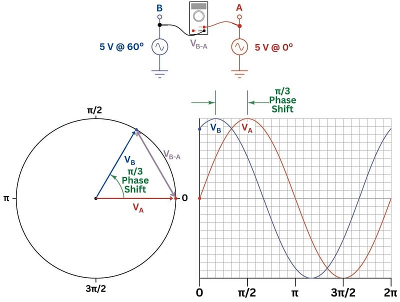
Phasor notation proves extremely useful to compare or combine AC quantities at the same frequency that are out-of-phase with each other. Consider the following example, showing two AC voltage waveforms of equal magnitude (5 volts peak) that are a constant 60 degrees (\(\pi \over 3\) radians) out of step with each other:
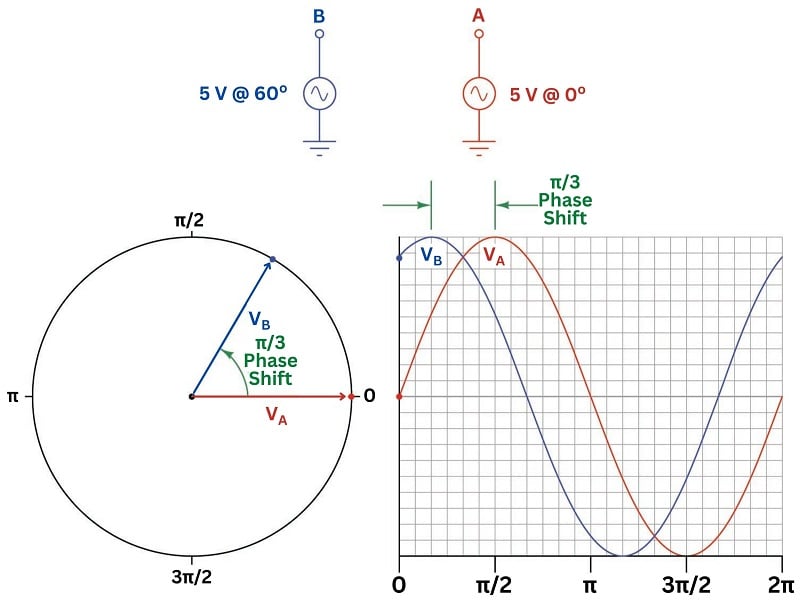
Recalling that the assumed direction of rotation for phasors is counter-clockwise, we see here that phasor \(B\) leads phasor \(A\) (i.e. phasor \(B\) is further counter-clockwise than phasor \(A\)). This is also evident from the rectangular graph, where we see sinusoid \(A\) lags behind sinusoid \(B\) by \(\pi \over 3\) radians. If we were to connect a dual-channel oscilloscope to these two voltage sources, we would see the same phase shift on its display.
Suppose we wished to calculate the amount of voltage between points B and A, sensing the difference in potential between these two AC voltage sources. Phasor notation makes this calculation rather easy to do, since all it entails is calculating the distance between the two phasor tips. We will designate this new measurement \(V_{BA}\) representing the potential at point B with reference to point A:
Simply sketching a new phasor stretching between the tips of phasors B and A yields a graphical solution for \(V_{BA}\). The length of phasor \(V_{BA}\) represents the magnitude of that voltage, while its angle from horizontal represents the phase shift of that voltage (compared to phasor A at 0\(^{o}\)).
If we wished to plot the sine wave represented by this new phasor, all we would have to do is move the \(V_{BA}\) phasor until its tail rested at the center of the circular graph (being careful to preserve its angle), then project its tip to the rectangular graph and plot the resulting wave through the new phasor’s complete rotation:
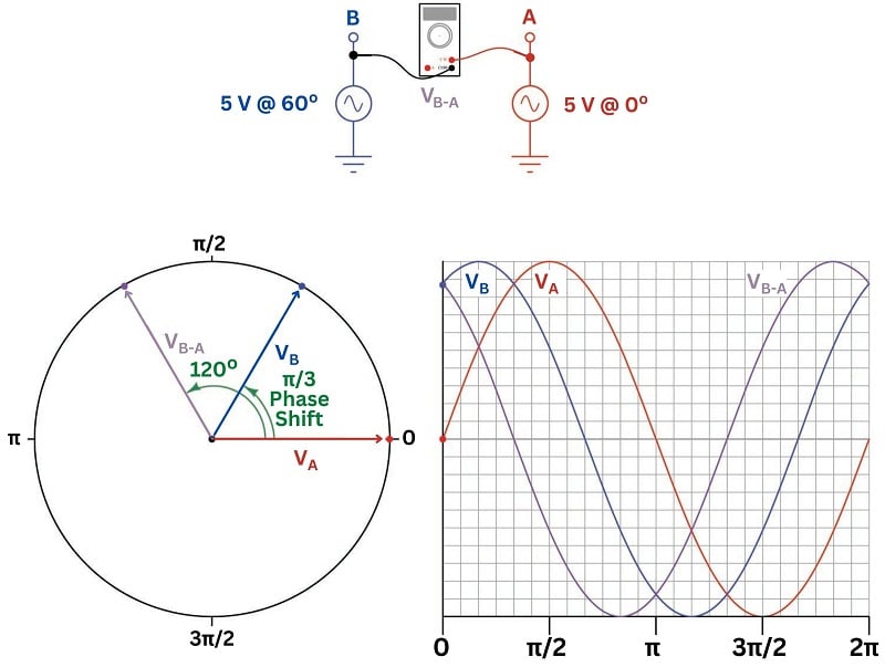
We see clearly now how phasor \(V_{BA}\) is phase-shifted 120\(^{}\) ahead of (leading) phasor A, and 60\(^{o}\) ahead of (leading) phasor B, possessing the same magnitude as both A and B. We may express each of these voltages in polar form:
\[V_A = 5 \hbox{ volts } \angle \> 0^{o}\]
\[V_B = 5 \hbox{ volts } \angle \> 60^{o}\]
\[V_{BA} = 5 \hbox{ volts } \angle \> 120^{o}\]
We may mathematically derive this result by subtracting \(V_A\) from \(V_B\) to arrive at \(V_{BA}\):
\[V_{BA} = V_B - V_A\]
\[(5 \hbox{ volts } \angle \> 60^{o}) - (5 \hbox{ volts } \angle \> 0^{o}) = 5 \hbox{ volts } \angle \> 120^{o}\]
When using phasors to describe differential voltages (i.e. voltages between two non-grounded points), it is important to specify which point is the reference. Suppose, for example, we took this same two-source system where each source has a peak voltage of 5 volts with reference to ground, but we connected our voltage-measuring instrument backwards from before such that the black (reference) lead touches point B and the red (measurement) lead touches point A (sensing \(V_{AB}\) instead of \(V_{BA}\)). Our new phasor \(V_{AB}\) must then be sketched with its tail (reference) at point B and its tip (measurement) at point A:
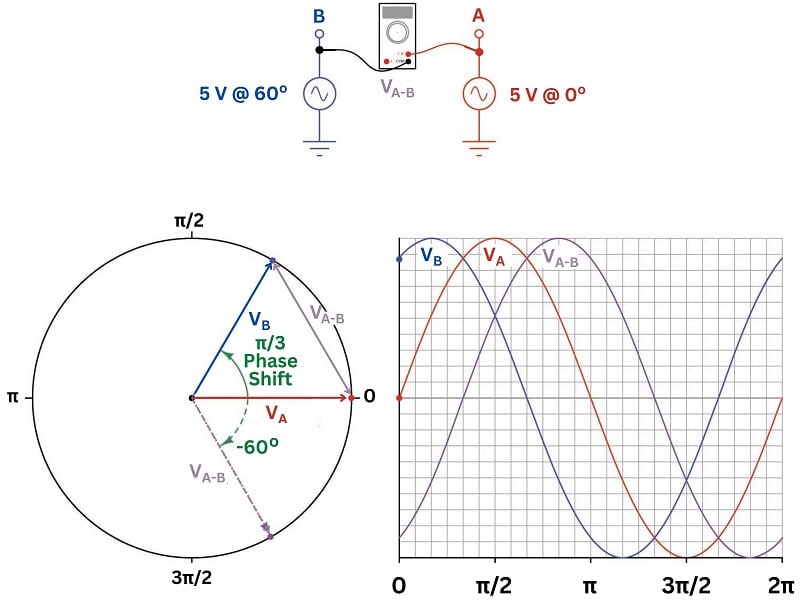
The dashed-line phasor is the same angle as the solid-line phasor reaching from point B to point A, just moved so that its tail rests at the circle’s center in order to plot its vertical projection on the rectangular graph to the right of the circle. As you can see, the new phasor \(V_{AB}\) is 180\(^{o}\) shifted from the old phasor \(V_{BA}\). This makes sense, as a reversal of the test leads on our voltage-sensing instrument must reverse the polarity of that voltage at every point in time.
We may mathematically derive this result by subtracting \(V_B\) from \(V_A\) to arrive at \(V_{AB}\):
\[V_{AB} = V_A - V_B\]
\[(5 \hbox{ volts } \angle \> 0^{o}) - (5 \hbox{ volts } \angle \> 60^{o}) = 5 \hbox{ volts } \angle \> -60^{o}\]
Thus, the new phasor \(V_{AB}\) actually lags behind both \(V_A\) (by 60 degrees) and \(V_B\) (by 120 degrees). If the voltage-sensing instrument is nothing more than a voltmeter, there will be no difference in its reading of \(V_{BA}\) versus \(V_{AB}\): in both cases it will simply register 5 volts AC peak. However, if the voltage-sensing instrument is an oscilloscope with its sweep triggered by one of the other voltage signals, this difference in phase will be clearly evident.
It is important to remind ourselves that voltage and current phasors, like the AC waveforms they represent, are actually in constant motion. Just as the generator shaft in an actual AC power system spins, the phasor representing that generator’s voltage and the phasor representing that generator’s current must also spin. The only way a phasor possessing a fixed angle makes any sense in the context of an AC circuit is if that phasor’s angle represents a relative shift compared to some other phasor at the same frequency. Here, we see Euler’s Relation written in fixed-angle and rotating-angle forms:
| Fixed-angle phasor | \(Ae^{j \theta} = A \cos \theta + j A \sin \theta\) |
|---|---|
| Rotating phasor | \(Ae^{j \omega t} = A \cos \omega t + j A \sin \omega t\) |
This concept can be very confusing, representing voltage and current phasors as possessing fixed angles when in reality they are continuously spinning at the system’s frequency. In order to make better sense of this idea, we will explore an analysis of the same two-source AC system using a special instrument designed just for the purpose.
Imagine building a small synchronous electric motor with an arrow-shaped magnetic rotor. We will wind the stator coils and magnetize the rotor such that the arrow points toward the 0\(^{o}\) mark whenever the red lead is positive and the black lead is negative (connected to a DC test source). When connected to an AC source, this phase meter, or “phasometer” will spin in sync with the AC generator powering the circuit, the rotating arrow keeping pace with the generator’s shaft. The intent of this arrow is to serve as a mechanical analog of an electrical phasor, pointing in the same direction as the phasor points for any sinusoidal voltage or current signal connected to the phasometer:
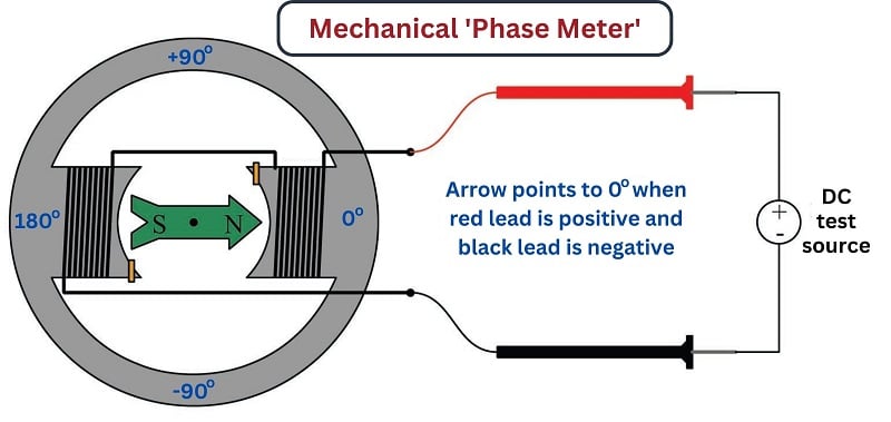
For a system frequency of 60 Hz as is standard for AC power systems in North America, the rotational speed of our phasometer’s rotor will be 3600 revolutions per minute – too fast for the rotating arrow to be anything but a blur of motion to an unaided human eye. Therefore, we will need to add one more component to the phasometer to make it practical: a strobe light connected to an AC voltage in the system to act as a synchronizing pulse. This strobe light will emit a flash of light just once per cycle of the AC waveform, and always at the same point in time (angle) within every cycle. Just as a strobe light (also called a “stroboscope”) makes a moving machine part appear to “freeze” in time, this strobe light will visually “freeze” the arrow so we will be able to read its position with our eyes.
Returning to our two-source AC system, we may perform a “thought experiment” to see what multiple phasometers would register if connected to various points in the system, using a single strobe light connected to source A (pulsing briefly every time its sensed voltage reaches the positive peak). Imagine this one strobe light is bright enough to clearly illuminate the faces of all phasometers simultaneously, visually “freezing” their arrows at the exact same point in every cycle:
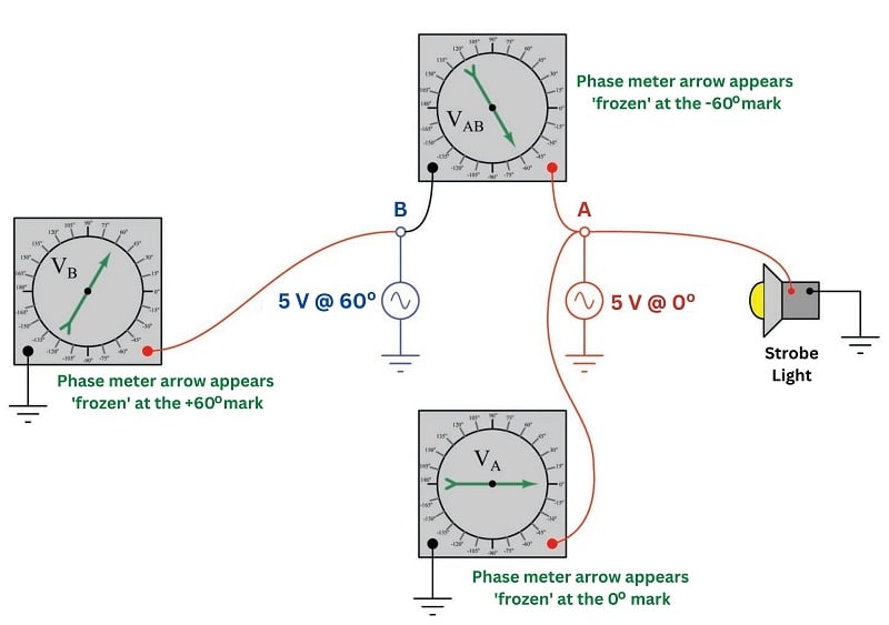
The phasometer connected to source A must register 0\(^{o}\) because the strobe light flashes whenever source A hits its positive peak (at 0\(^{o}\) on its cosine waveform), and the positive peak of a waveform is the precise point at which the phasometer arrow is designed to orient itself toward the 0\(^{o}\) mark. The phasometer connected to source B will register 60\(^{o}\) because that source is 60 degrees ahead of (leading) source A, having passed its positive peak already and now headed downward toward zero volts at the point in time when the strobe flashes. The upper phasometer registers \(-60^{o}\) at that same time because the voltage it senses at point A with respect to point B is lagging behind source A by that much, the \(V_{AB}\) cosine wave heading toward its positive peak.
If we were to substitute a constant illumination source for the strobe light, we would see all three phasometers’ arrows spinning counter-clockwise, revealing the true dynamic nature of the voltage phasors over time. Remember that these phasors are all continuously moving quantities, because the voltages they represent are sinusoidal functions of time. Only when we use a strobe light keyed to source A’s positive peak do we see fixed-angle readings of \(V_A = 0^{o}\), \(V_B = 60^{o}\), and \(V_{AB} = -60^{o}\).
You may wonder what might happen if we keep the three phasometers connected to the same points, but change the strobe light’s reference point. The answer to this question is that the new reference source voltage will now be our zero-degree definition, with every phasor’s angle changing to match this new reference. We may see this effect here, using the same two sources and three phasometers, but moving the strobe light from source A to source B:
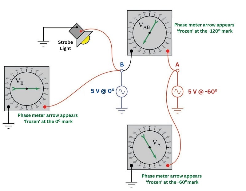
Having the strobe light keyed to source B makes it flash 60 degrees earlier than it did when it was keyed to source A, which in turn “freezes” the arrows on the faces of all three phasometers \(-60^{o}\) from where they used to be when source A was the time-reference. The following table compares the phasometer readings with both strobe light reference points:
| Strobe reference | \(V_A\) | \(V_B\) | \(V_{AB}\) |
|---|---|---|---|
| Source A | 0\(^{o}\) | 60\(^{0}\) | \(-60^{o}\) |
| Source B | \(-60^{o}\) | 0\(^{0}\) | \(-120^{o}\) |
It is even possible to imagine connecting the strobe light to a special electronic timing circuit pulsing the light at 60 Hz (the AC system’s frequency), synchronized to an atomic clock so as to keep ultra-accurate time. Such an arrangement would permit phasor angle measurements based on an absolute time reference (i.e. the atomic clock) rather than a relative time reference (i.e. one of the AC voltage sources). So long as the two AC sources maintained the same frequency and phase shift, the three phasometers would still be displaced 60\(^{o}\) from each other, although it would only be by blind luck that any of them would point toward 0\(^{o}\) (i.e. that any one voltage would happen to be precisely in-phase with the electronic timer circuit’s 60 Hz pulse).
Interestingly, this technique of measuring AC power system phasors against an absolute time reference is a real practice and not just a textbook thought experiment. The electrical power industry refers to this as a synchrophasor measurement. Special instruments called Phasor Measurement Units or PMUs connect to various points within the power system to acquire real-time voltage and current measurements, each PMU also connected to a GPS (Global Positioning System) radio receiver to obtain an absolute time reference with sub-microsecond uncertainty. Each PMU uses the ultra-precise time signal from the GPS receiver to synchronize a “standard” cosine wave at the power system frequency such that this reference waveform is at its positive peak (0\(^{o}\)) at the top of every second in time.
Synchrophasor technology makes it possible to perform simultaneous comparisons of phasor angles throughout a power system, which is useful for such tasks as analyzing frequency stability in a power grid or detecting “islanding” conditions where tripped circuit breakers segment a power grid and allow distributed generators to begin drifting out of sync with each other.
Phasors and Impedance
The ultimate purpose of phasors is to simplify AC circuit analysis, so this is what we will explore now. Consider the problem of defining electrical opposition to current in an AC circuit. In DC (direct-current) circuits, resistance (\(R\)) is defined by Ohm’s Law as being the ratio between voltage (\(V\)) and current (\(I\)):
\[R = {V \over I}\]
There are some electrical components, though, which do not obey Ohm’s Law. Capacitors and inductors are two outstanding examples. The fundamental reason why these two components do not follow Ohm’s Law is because they do not dissipate energy like resistances do. Rather than dissipate energy (in the form of heat and/or light), capacitors and inductors store and release energy from and to the circuit in which they are connected. The contrast between resistors and these components is remarkably similar to the contrast between friction and inertia in mechanical systems. Whether pushing a flat-bottom box across a floor or pushing a heavy wheeled cart across a floor, work is required to get the object moving. However, the flat-bottom box will immediately stop when you stop pushing it due to the energy loss inherent to friction, while the wheeled cart will continue to coast because it has kinetic energy stored in it. When a resistor disconnected from an electrical source, both voltage and current immediately cease. Capacitors and inductors, however, may store a “charge” of energy when disconnected from a source (capacitors retaining voltage and inductors retaining current).
The relationships between voltage and current for capacitors (\(C\)) and inductors (\(L\)) are as follows:
\[I = C {dV \over dt}\]
\[V = L {dI \over dt}\]
Expressed verbally, capacitors pass electric current proportional to how quickly the voltage across them changes over time. Conversely, inductors produce a voltage drop proportional to how quickly current through them changes over time. The symmetry here is beautiful: capacitors, which store energy in an electric field that is proportional to the applied voltage, oppose changes in voltage. Inductors, which store energy in a magnetic field that is proportional to applied current, oppose changes in current. The manner in which a capacitor or an inductor reacts to changes imposed upon it is a direct consequence of the Law of Energy Conservation: since energy can neither appear from nothing nor simply vanish, an exchange of energy must take place in order to alter the amount of energy stored within a capacitor or an inductor. The rate at which a capacitor’s voltage may change is directly related to the rate at which electric charge (current) enters or exits the capacitor. The rate at which an inductor’s current may change is directly related to the amount of electromotive force (voltage) impressed across the inductor.
When either type of component is placed in an AC circuit and subjected to oscillating signals, it will pass a finite amount of alternating current. Even though the mechanism of a capacitor’s or inductor’s opposition to current (called reactance) is fundamentally different from that of a resistor (called resistance), just like inertia differs in its fundamental nature from friction, it is still convenient to express the amount of electrical opposition in a common unit of measurement: the ohm (\(\Omega\)). To do this, we will have to figure out a way to take the above equations and manipulate them to express each component’s behavior as a ratio of \(V \over I\).
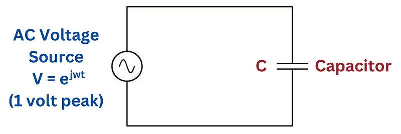
Let’s start with capacitors. Suppose we impress a 1 volt peak AC voltage across a capacitor, representing that voltage as the exponential \(e^{j \omega t}\) where \(\omega\) is the angular velocity (frequency) of the signal and \(t\) is time:
We will begin by writing the current/voltage relationship for a capacitor, along with the imaginary exponential function for the impressed voltage:
\[I = C {dV \over dt} \hskip1em \hbox{where} \hskip1em V = e^{j \omega t}\]
Substituting \(e^{j \omega t}\) for \(V\) in the capacitor formula, we see we must apply the calculus function of differentiation to the time-based voltage function:
\[I = C {d \over dt} \left( e^{j \omega t} \right)\]
Fortunately for us, differentiation is a very simple process with exponential functions:
\[I = j \omega C e^{j \omega t}\]
Remember that our goal here is to solve for the ratio of voltage over current for a capacitor. So far all we have is a function for current (\(I\)) in terms of time (\(t\)). If we take this function for current and divide that into our original function for voltage, however, we see that ratio simplify quite nicely:
\[{V \over I} = {{e^{j \omega t}} \over {j \omega C e^{j \omega t}}}\]
\[{V \over I} = {1 \over {j \omega C}} = -j {1 \over {\omega C}}\]
Note how the exponential term completely drops out of the equation, leaving us with a clean ratio strictly in terms of capacitance (\(C\)), angular velocity (\(\omega\)), and of course \(j\).
Next, we will apply this same analysis to inductors. Recall that voltage across an inductor and current through an inductor are related as follows:
\[V = L {dI \over dt}\]
If we describe the AC current through an inductor using the familiar imaginary exponential expression \(I = e^{j \omega t}\) (representing a 1 amp peak AC current at frequency \(\omega\)), we may substitute this expression for current into the inductor’s characteristic equation to solve for the inductor’s voltage as a function of time:
\[V = L {dI \over dt} \hskip1em \hbox{where} \hskip1em I = e^{j \omega t}\]
\[V = L {d \over dt} \left( e^{j \omega t} \right)\]
\[V = j \omega L e^{j \omega t}\]
Now that we have the inductor’s voltage expressed as a time-based function, we may include the original current function and calculate the ratio of \(V\) over \(I\):
\[{V \over I} = {{j \omega L e^{j \omega t}} \over {e^{j \omega t}}}\]
\[{V \over I} = j \omega L\]
In summary, we may express the impedance (voltage-to-current ratio) of capacitors and inductors by the following equations:
\[ Z_C = {1 \over j \omega C} \hskip1em \hbox{or} \hskip1em -j {1 \over {\omega C}}\]
\[Z_L = j \omega L\]
Most students familiar with electronics from an algebraic perspective (rather than calculus) find the expressions \(X_L = 2 \pi f L\) and \(X_C = {1 \over 2 \pi f C}\) easier to grasp. Just remember that angular velocity (\(\omega\)) is really “shorthand” notation for \(2 \pi f\), so these familiar expressions may be alternatively written as \(X_L = \omega L\) and \(X_C = {1 \over \omega C}\).
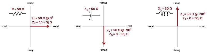
Furthermore, recall that reactance (\(X\)) is a scalar quantity, having magnitude but no direction. Impedance (\(Z\)), on the other hand, possesses both magnitude and direction (phase), which is why the imaginary operator \(j\) must appear in the impedance expressions to make them complete. The impedance offered by pure inductors and capacitors alike are nothing more than their reactance values (\(X\)) scaled along the imaginary (\(j\)) axis (phase-shifted 90\(^{o}\)).
These different representations of opposition to electrical current are shown here for components exhibiting 50 ohms, resistances (\(R\)) and reactances (\(X\)) shown as scalar quantities near the component symbols, and impedances (\(Z\)) as phasor quantities on the complex plane:
Phasor Math
Another detail of phasor math that is both beautiful and practical is the famous expression of Euler’s Relation, the one all math teachers love because it directly relates several fundamental constants in one elegant equation (remember that \(i\) and \(j\) mean the same thing, just different notational conventions for different disciplines):
\[e^{i \pi} = -1\]
This equation is actually a special case of Euler’s Relation, relating imaginary exponents of \(e\) to sine and cosine functions:
\[e^{i\theta} = \cos \theta + i \sin \theta\]
What this equation says is really quite amazing: if we raise \(e\) to an imaginary exponent of some angle (\(\theta\)), it is equivalent to the real cosine of that same angle plus the imaginary sine of that same angle. Thus, Euler’s Relation expresses an equivalence between exponential (\(e^x\)) and trigonometric (\(\sin x\), \(\cos x\)) functions. Specifically, the angle \(\theta\) describes which way a phasor points on a complex plane, the real and imaginary coordinates of a unit phasor’s tip being equal to the cosine and sine values for that angle, respectively.
If we set the angle \(\theta\) to a value equal to \(\pi\), we see the general form of Euler’s relation transform into \(e^{i \pi} = -1\):
\[e^{i\theta} = \cos \theta + i \sin \theta\]
\[e^{i\pi} = \cos \pi + i \sin \pi\]
\[e^{i\pi} = -1 + i0\]
\[e^{i\pi} = -1\]
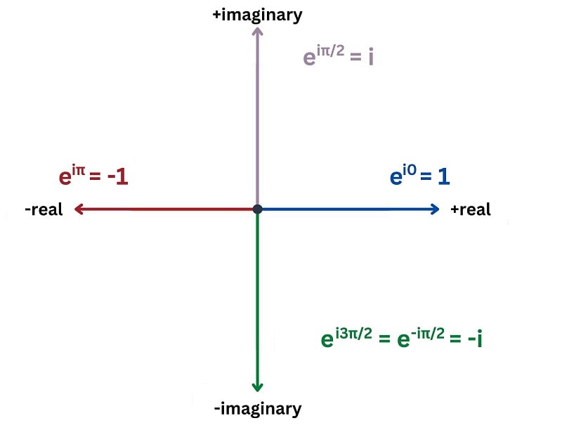
After seeing this, the natural question to ask is what happens when we set \(\theta\) equal to other, common angles such as 0, \(\pi \over 2\), or \(3\pi \over 2\) (also known as \(-{\pi \over 2}\))? The following examples explore these angles:
| Angle (\(\theta\)) | Exponential | Trigonometric | Rectangular | Polar |
|---|---|---|---|---|
| 0 radians = 0\(^{o}\) | \(e^{i0}\) | \(\cos 0 + i \sin 0\) | \(1 + i0 = 1\) | 1 \(\angle\) 0\(^{o}\) |
| \(\pi / 2\) radians = 90\(^{o}\) | \(e^{i \pi / 2}\) | \(\cos 90^{o} + i \sin 90^{o}\) | \(0 + i1 = i\) | 1 \(\angle\) 90\(^{o}\) |
| \(\pi\) radians = 180\(^{o}\) | \(e^{i \pi}\) | \(\cos 180^{o} + i \sin 180^{o}\) | \(-1 + i0 = -1\) | 1 \(\angle\) 180\(^{o}\) |
| \(-\pi / 2\) radians = \(-\)90\(^{o}\) | \(e^{i -\pi / 2}\) | \(\cos -90^{o} + i \sin -90^{o}\) | \(0 - i1 = -i\) | 1 \(\angle\) \(-\)90\(^{o}\) |
We may show all the equivalences on the complex plane, as unit phasors:
As we saw previously, the amount of opposition to electrical current offered by reactive components (i.e. inductors and capacitors) – a quantity known as impedance – may be expressed as functions of \(j\) and \(\omega\):
\[Z_L = j \omega L\]
\[Z_C = -j {1 \over \omega C}\]
Knowing that \(j\) is equal to \(e^{j \pi / 2}\) and that \(-j = e^{- j \pi / 2}\), we may re-write the above expressions for inductive and capacitive impedance as functions of an angle:
\[Z_L = \omega L e^{j \pi /2}\]
\[Z_C = {1 \over \omega C} e^{- j \pi /2}\]
Using polar notation as a “shorthand” for the exponential term, the impedances for inductors and capacitors are seen to have fixed angles:
\[Z_L \hskip 5pt = \hskip 5pt \omega L e^{j \pi /2} \hskip 5pt = \hskip 5pt \omega L \angle {\pi \over 2} \hbox{ radians} \hskip 5pt = \hskip 5pt \omega L \angle 90^{o}\]
\[Z_C \hskip 5pt = \hskip 5pt {1 \over \omega C} e^{- j \pi /2} \hskip 5pt = \hskip 5pt {1 \over \omega C} \angle -{\pi \over 2} \hbox{ radians} \hskip 5pt = \hskip 5pt {1 \over \omega C} \angle -90^{o}\]
Beginning electronics students will likely find the following expressions of inductive and capacitive impedance more familiar, \(2 \pi f\) being synonymous with \(\omega\):
\[Z_L = (2 \pi f L) \angle 90^{o}\]
\[Z_C = \left({1 \over 2 \pi f C}\right) \angle -90^{o}\]
The beauty of complex numbers in AC circuits is that they make AC circuit analysis equivalent to DC circuit analysis. If we represent every voltage and every current and every impedance quantity in an AC circuit as a complex number, all the same laws and rules we know from DC circuit analysis will apply to the AC circuit. This means we need to be able to add, subtract, multiply, and divide complex numbers in order to apply Ohm’s Law and Kirchhoff’s Laws to AC circuits.
The basic rules of phasor arithmetic are listed here, with phasors having magnitudes of \(A\) and \(B\), and angles of \(M\) and \(N\), respectively:
\[Ae^{jM} + Be^{jN} = (A \cos M + B \cos N) + j (A \sin M + B \sin N)\]
\[Ae^{jM} - Be^{jN} = (A \cos M - B \cos N) + j (A \sin M - B \sin N)\]
\[Ae^{jM} \times Be^{jN} = ABe^{j(M + N)}\]
\[Ae^{jM} \div Be^{jN} = {A \over B} \left[ e^{j(M - N)} \right]\]
Addition and subtraction lend themselves readily to the rectangular form of phasor expression, where the real (cosine) and imaginary (sine) terms simply add or subtract. Multiplication and division lend themselves readily to the polar form of phasor expression, where magnitudes multiply or divide and angles add or subtract.
To summarize:
- Voltages and currents in AC circuits may be mathematically represented as phasors, which are imaginary exponential functions (\(e\) raised to imaginary powers)
- Phasors are typically written in either rectangular form (real + imaginary) or polar form (magnitude @ angle)
- Ohm’s Law and Kirchhoff’s Laws still apply in AC circuits as long as all quantities are in phasor notation
- Addition is best done in rectangular form: add the real parts, and add the imaginary parts
- Subtraction is best done in rectangular form: subtract the real parts, and subtract the imaginary parts
- Multiplication is best done in polar form: multiply the magnitudes, and add the angles
- Division is best done in polar form: divide the magnitudes, and subtract the angles
It should be noted that many electronic calculators possess the ability to perform all these arithmetic functions in complex-number form. If you have access to such a calculator, it will greatly simplify any AC circuit analysis performed with complex numbers!
AC Circuit Analysis Using Phasors
A phasor is a special form of vector (a quantity possessing both magnitude and direction) lying in a complex plane. Phasors relate circular motion to simple harmonic (sinusoidal) motion as shown in the following diagram. In AC electrical circuits, this is the relationship between an electromechanical generator’s shaft angle and the sinusoidal voltage it outputs:
In any operating AC electrical circuit the phasors, just like the sinusoidal waveforms, never rest: they are in continuous motion. When we speak of a phasor as having a fixed angle, what we really mean is that the phasor is either leading or lagging with respect to some other “reference” phasor in the system, not that the phasor itself is stationary. We explored this concept previously, where we used an invented instrument called a “phasometer” to represent the direction of a measured phasor in real time, and then used a strobe light connected to some point in the same system to visually “freeze” the phasometer arrows so we could see which direction each arrow was pointed at the moment in time when our chosen reference waveform reached its positive peak value (i.e. 0\(^{o}\) on a cosine wave). The fixed angle represented by each “strobed” phasometer arrow therefore represented the amount of relative phase shift between each respective phasor and the reference phasor.
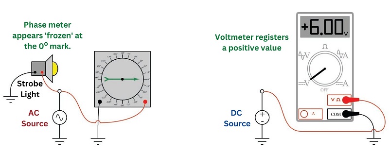
Phasor angles are to AC quantities what arithmetic signs are to DC quantities. If a phasometer registers an angle of 180 degrees, it means the red lead is fully negative and the black lead is fully positive at the moment in time when the strobe light flashes. If a DC voltmeter registers a negative voltage, it means the red lead is negative and the black lead is positive at the time of the measurement:
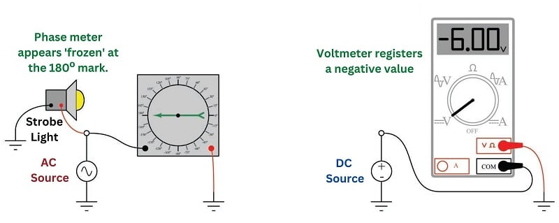
Reversing each instrument’s test lead connections to the circuit will reverse its indication: flipping red and black leads on the phasometer will cause its indication to be 0\(^{o}\) instead of 180\(^{o}\) ; flipping red and black leads on the DC voltmeter will cause it to register a positive voltage instead of a negative voltage:
From these demonstrations we can see that the indication given by a measuring instrument depends as much on how that instrument connects to the circuit as it does on the circuit quantity itself. Likewise, a voltage or current value obtained in the course of analyzing a circuit depends as much on how we label the assumed polarity (or direction) of that quantity on the diagram as it does on the quantity itself.
To illustrate the importance of signs, assumed directions, and phasor angles in circuit analysis, we will consider two multi-source circuits: one DC and one AC. In each case we will explore how Kirchhoff’s Current Law relates to currents at a similar node in each circuit, relating the current arrow directions to signs and phasor angles.
First, the DC circuit:
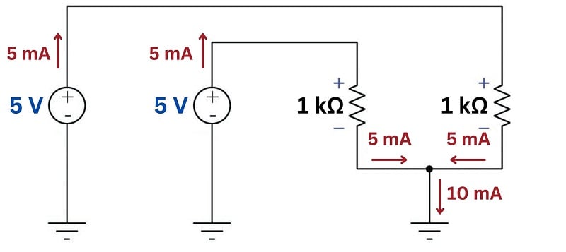
With each 1 k\(\Omega\) resistor powered by its own 5 volt DC source, the current through each of these resistors will be 5 milliamps in accordance with Ohm’s Law (\(I = {V \over R}\)). The direction of each current is easily predicted by examining the polarity of each source (with current represented in conventional flow notation exiting the positive terminal and entering the negative terminal of each source) and/or by examining the polarity of the voltage drop across each resistor (with conventional-flow current entering the positive terminal and exiting the negative terminal of each load). At the node below the two resistors, these two currents join together to form a larger (10 milliamp) current headed toward ground. Kirchhoff’s Current Law declares that the sum of all currents entering a node must equal the sum of all currents exiting that node. Here we see this is true: 5 milliamps in plus 5 milliamps in equals 10 milliamps out.
The voltage polarities and current directions in this DC circuit are all clear and unambiguous because the quantities are constant over time. Each power supply acts as an energy source and each resistor acts as an energy load, all the time. Our application of Kirchhoff’s Current Law at the node is so obvious it hardly requires explanation: the flow of charge carriers (current) in and out must be in equilibrium.
With AC, however, we know things will not be so simple. AC circuit quantities are not constant over time as they are in DC circuits. Reactive (energy-storing) components such as inductors and capacitors play alternating roles as sources and loads, complicating their analysis. The good news in all of this is that phasor representations of voltage and current allow us to apply all the same fundamental principles we are accustomed to using for DC circuits (e.g. Ohm’s Law, Kirchhoff’s Voltage Law, Kirchhoff’s Current Law, network theorems, etc.). In order to use these principles to calculate AC quantities, though, we must be careful in how we label them in the circuit.
Here, we will modify the circuit to include two AC power sources (phase-shifted by 60\(^{o}\)), and replace one of the 1 k\(\Omega\) resistors with a capacitor exhibiting 1 k\(\Omega\) of reactance at the system frequency. As in the DC circuit, each of the two loads sees the full 5 volts of its respective source. Unlike the DC circuit, we must represent each of the voltage and impedance quantities in complex (phasor) form in order to apply Ohm’s Law to calculate load currents.
One more thing we will do to this circuit before beginning any phasor arithmetic is to label each voltage and each current as we did in the DC circuit. Placing + and \(-\) symbols at the terminals of AC voltage sources, and drawing conventional-flow notation arrows showing alternating current through loads at first may seem absurd, since we know this is an AC circuit and so by definition these quantities lack fixed polarities and directions. However, these symbols will become very important to us because they serve to define what 0\(^{o}\) means for each of the respective phasors. In other words, these polarities and arrows merely show us which way the voltages and currents are oriented when each of those phasors is at its positive peak – i.e. when each phasor angle comes around to its own 0\(^{o}\) mark. As such, the polarities and arrows we draw do not necessarily represent simultaneous conditions. We will rely on the calculated phasor angles to tell us how far these quantities will actually be phase-shifted from each other at any given point in time:
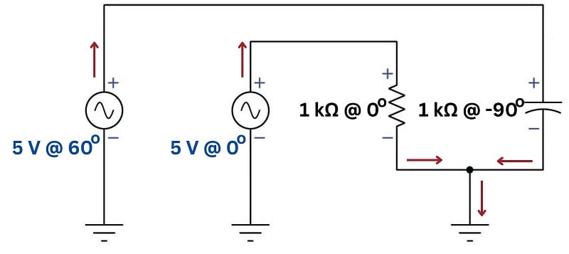
First, calculating current through the resistor, recalling that the impedance of a resistor has a 0 degree phase angle (i.e. no phase shift between voltage and current):
\[I_R = {V_R \over Z_R} = {5 \hbox{ V} \angle \> 0^{o} \over 1 \hbox{ k}\Omega \angle \> 0^{o}} = 5 \hbox{ mA} \angle \> 0^{o}\]
Next, calculating current through the capacitor, recalling that the impedance for a capacitor has a \(-\)90 degree phase angle because voltage across a capacitor lags 90 degrees behind current through a capacitor:
\[I_C = {V_C \over Z_C} = {5 \hbox{ V} \angle \> 60^{o} \over 1 \hbox{ k}\Omega \angle \> -90^{o}} = 5 \hbox{ mA} \angle \> 150^{o}\]
From the arrows sketched at the node we can see the total current headed toward ground must be equal to the sum of the two currents headed into the node, just as with the DC circuit. The difference here is that we must perform the addition using phasor quantities instead of scalar quantities in order to account for phase shift between the two currents:
\[I_{total} = I_R + I_C\]
\[I_{total} = 5 \hbox{ mA} \angle \> 0^{o} + 5 \hbox{ mA} \angle \> 150^{o}\]
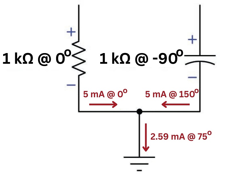
Representing these current phasors in rectangular mode so we may sum their real and imaginary parts:
\[I_{total} = (5 + j 0 \hbox{ mA}) + (-4.33 + j 2.5 \hbox{ mA})\]
\[I_{total} = 0.67 + j 2.5 \hbox{ mA}\]
Converting the rectangular form into polar form:
\[I_{total} = 2.59 \hbox{ mA} \angle \> 75^{o}\]
This result is highly non-intuitive. When we look at the circuit and see two 5 milliamp currents entering a node, we naturally expect a sum total of 10 milliamps to exit that node. However, that will only be true if those 5 mA quantities are simultaneous: i.e. if the two currents are 5 mA in magnitude at the same point in time. Since we happen to know these two currents are phase-shifted from each other by 150 degrees (nearly opposed to each other), they never reach their full strength at the same point in time, and so their sum is considerably less than 10 milliamps:
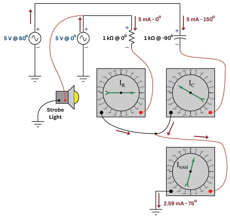
We may make more sense of this result by adding current-sensing phasometers to the circuit, their red and black test leads connected in such a way as to match the arrows’ directions (current entering the red lead and exiting the black lead, treating the phasometer as a proper electrical load) as though these were DC ammeters being connected into a DC circuit:
A very common and practical example of using “DC notation” to represent AC voltages and currents is in three-phase circuits where each power supply consists of three AC voltage sources phase-shifted 120 degrees from each other. Here, we see a “wye” connected generator supplying power to a “wye” connected load. Each of the three generator stator windings outputs 277 volts, with the entirety of that voltage dropped across each of the load resistances:
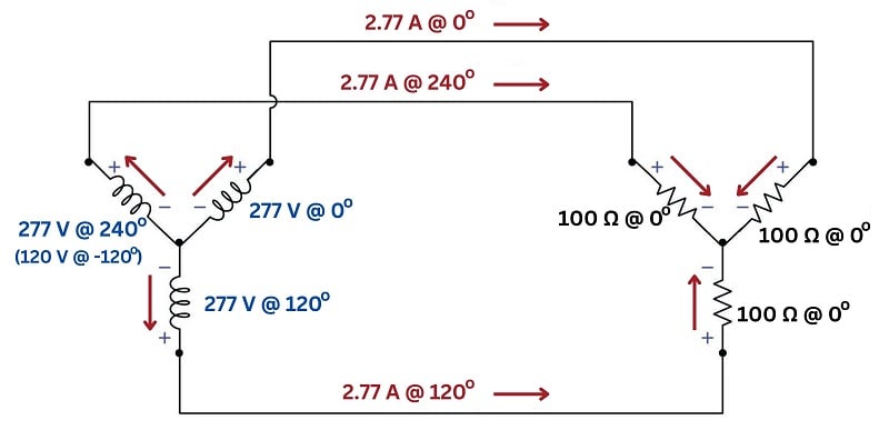
Note the directions of the three currents (red arrows) in relation to the node at the center of the generator’s “wye” winding configuration, and also in relation to the node at the center of the resistive load’s “wye” configuration. At first this seems to be a direct violation of Kirchhoff’s Current Law: how is it possible to have three currents all exiting a node with none entering or to have three currents all entering a node with none exiting? Indeed, this would be impossible if the currents were simultaneously moving in those directions, but what we must remember is that each of the current arrows simply shows which way each current will be moving when its respective phasor comes around to the 0\(^{o}\) mark. In other words, the arrows simply define what zero degrees means for each current. Similarly, the voltage polarities would suggest to anyone familiar with Kirchhoff’s Voltage Law in DC circuits that the voltage existing between any two of the power conductors between generator and load should be 0 volts, reading the series-opposed sum of two 277 volt sources. However, once again we must remind ourselves that the + and \(-\) symbols do not actually represent polarities at the same point in time, but rather serve to define the orientation of each voltage when its phasor happens to point toward 0\(^{o}\).
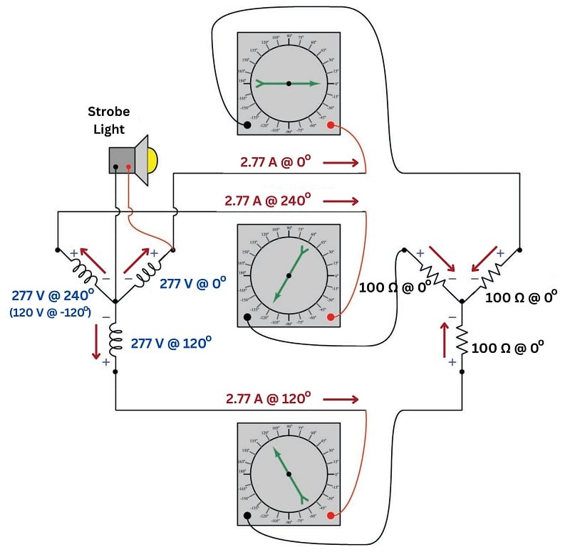
If we were to connect three current-sensing phasometers to measure the phase angle of each line current in this system (keying the strobe light to the voltage of the 0\(^{o}\) generator winding), we would see the true phase relationships relative to that time reference. The directions of the current arrows and the orientation of the + and \(-\) polarity marks serve as references for how we shall connect the phasometers to the circuit (+ on red, \(-\) on black; current entering red, exiting black):
We may use the three arrows at the load’s center node to set up a Kirchhoff’s Current Law equation (i.e. the sum of all currents at a node must equal zero), and confirm that the out-of-phase currents all “entering” that node do indeed amount to a sum of zero:
\[I_{node} = 2.77 \hbox{ A} \angle 0^{o} + 2.77 \hbox{ A} \angle 120^{o} + 2.77 \hbox{ A} \angle 240^{o}\]
Converting polar expressions into rectangular so we may see how they add together:
\[I_{node} = (2.77 + j 0 \hbox{ A}) + (-1.385 + j 2.399 \hbox{ A}) + (-1.385 - j 2.399 \hbox{ A})\]
Combining all the real terms and combining all the imaginary terms:
\[I_{node} = (2.77 - 1.385 - 1.385) + j(0 + 2.399 - 2.399) \hbox{ A}\]
\[I_{node} = 0 + j 0 \hbox{ A}\]
Looking closer at these results, we may determine which way the three currents were actually flowing at the time of the strobe’s flash (when the upper-right generator winding is at its peak positive voltage). The first phasor has a real value of +2.77 amps at that instant in time, which represents 2.77 amps of actual current flowing in the actual direction of our sketched current arrow. The second and third phasors each have real values of \(-\)1.385 amps at that same instant in time, representing 1.385 amps each flowing against the direction of our sketched arrows (i.e. leaving that node). Thus, we can see that the “snapshot” view of currents at the time of the strobe’s flash makes complete sense: one current of 2.77 amps entering the node and two currents of 1.385 amps each exiting the node. Viewed at any instant in time, the principles of DC circuits hold true. It is only when we sketch polarity marks and draw arrows representing voltages and currents reaching their positive peak values at different times that the annotations seem to violate basic principles of circuit analysis.
REVIEW:
-
Circular power generation yields a continuous positive and negative (sine wave) pattern.
-
When capacitors and inductors are used in an AC circuit, they introduce advances and delays, respectively, on the peak of current versus voltage (phase shift).
-
Resistance is observed on the positive ‘real’ axis, with no phase shift.
-
Capacitors are observed on the negative ‘imaginary’ axis, with current peaking just before voltage.
-
Inductors are observed on the positive ‘imaginary’ axis, with current peaking just after voltage.
-
Phasors are the trigonometric relationship between the sine waveform and these introduced phase shifts, allowing us to determine the actual flow of current in any part of the circuit.
