 Facebook
 Google
 GitHub
 Linkedin
The Concept of Differentiation
Suppose we wished to measure the rate of propane gas flow through a hose to a torch:
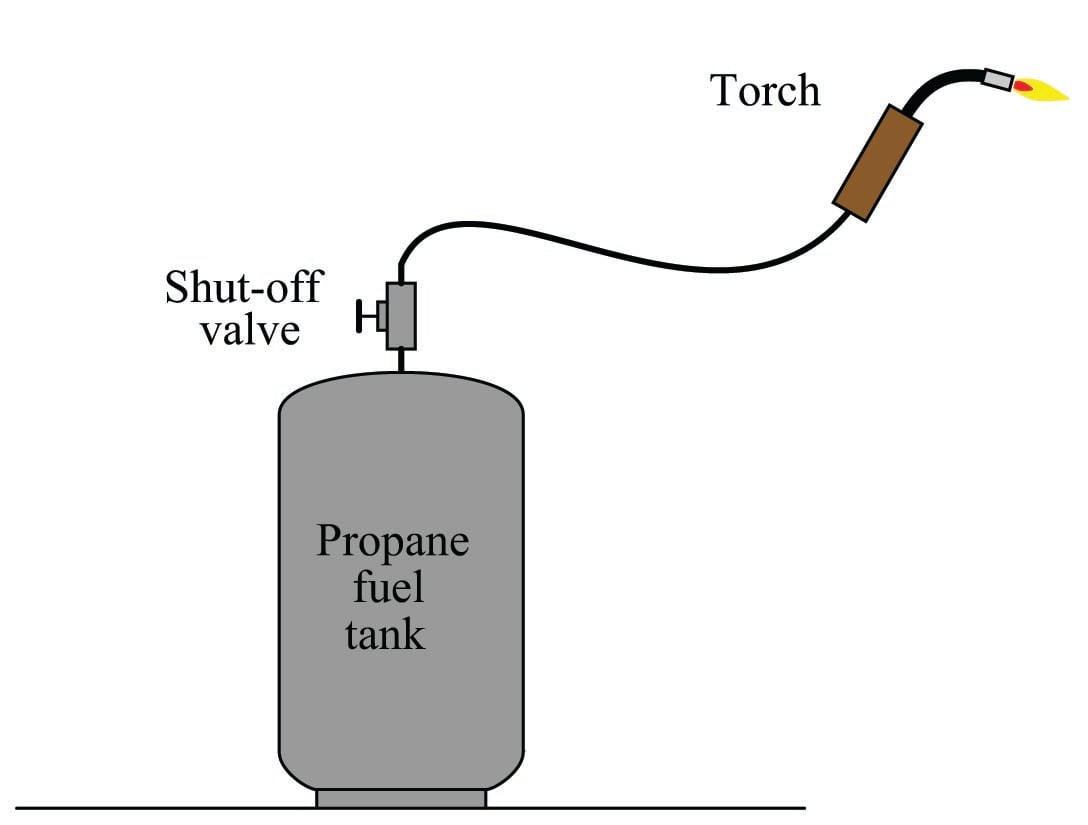
Flowmeters appropriate for measuring low flow rates of any gas are typically very expensive, making it impractical to directly measure the flow rate of propane fuel gas consumed by this torch at any given moment. We could, however, indirectly measure the flow rate of propane by placing the tank on a scale where its mass (\(m\)) could be monitored over time. By taking measurements of mass over short time periods (\(\Delta t\)), we could calculate the corresponding differences in mass (\(\Delta m\)), then calculate the ratio of mass lost over time to calculate average mass flow rate (\(\overline{W}\)):
\[\overline{W} = {\Delta m \over \Delta t} = \hbox{Average mass flow rate}\]
Where,
\(\overline{W}\) = Average mass flow rate within each time period (kilograms per minute)
\(\Delta m\) = Measured mass difference over time period (kilograms)
\(\Delta t\) = Time period of mass measurement sample (minutes)
Note that flow rate is a ratio (quotient) of mass change over time change. The units used to express flow even reflect this process of division: kilograms per minute.
\[\overline{W} = {\hbox{[kg]} \over \hbox{[min]}} = \hbox{Average mass flow rate} = \left[{\hbox{kg} \over \hbox{min}}\right]\]
Graphed as a function over time, the tank’s mass will be seen to decrease as time elapses. Each dot represents a mass and time measurement coordinate pair (e.g. 20 kilograms at 7:38, 18.6 kilograms at 7:51, etc.):
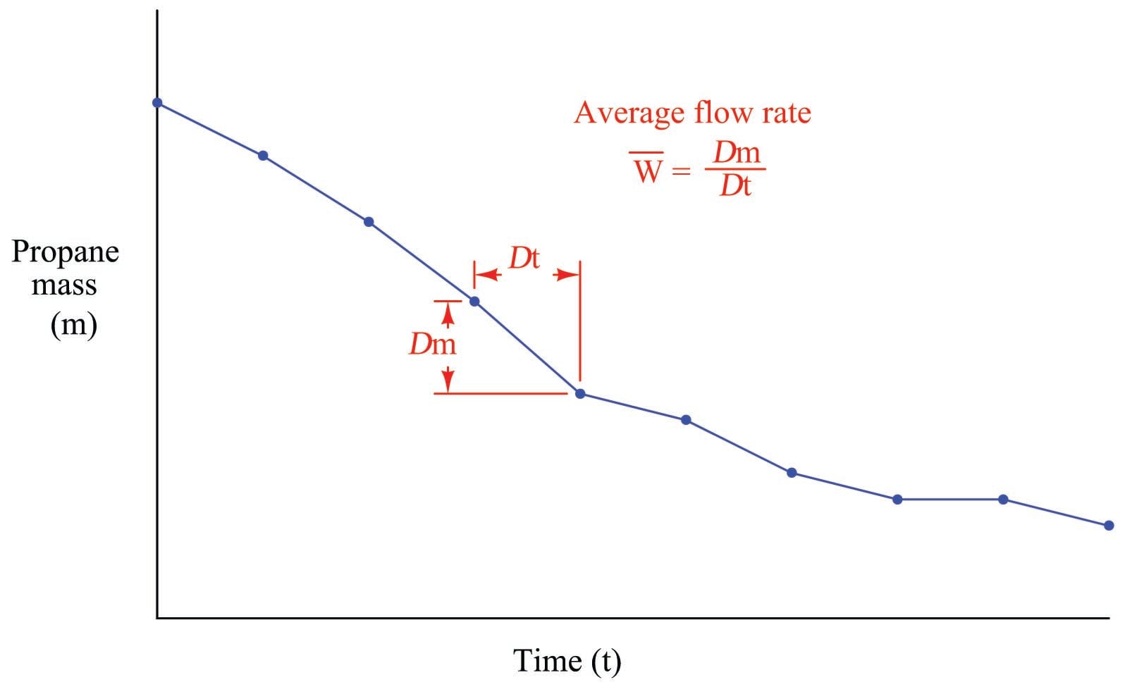
We should recall from basic geometry that the slope of a line or line segment is defined as its rise (vertical height) divided by its run (horizontal width). Thus, the average mass flow rate calculated within each time period may be represented as the pitch (slope) of the line segments connecting dots, since mass flow rate is defined as a change in mass per (divided by) change in time.
Periods of high propane flow (large flame from the torch) show up on the graph as steeply-pitched line segments. Periods of no propane flow reveal themselves as flat portions on the graph (no rise or fall over time).
If the determination of average flow rates between significant gaps in time is good enough for our application, we need not do anything more. However, if we wish to detect mass flow rate at any particular instant in time, we need to perform the same measurements of mass loss, time elapse, and division of the two at an infinitely fast rate.
Supposing such a thing were possible, what we would end up with is a smooth graph showing mass consumed over time. Instead of a few line segments roughly approximating a curve, we would have an infinite number of infinitely short line segments connected together to form a seamless curve. The flow rate at any particular point in time would be the ratio of the mass and time differentials (the slope of the infinitesimal line segment) at that point:
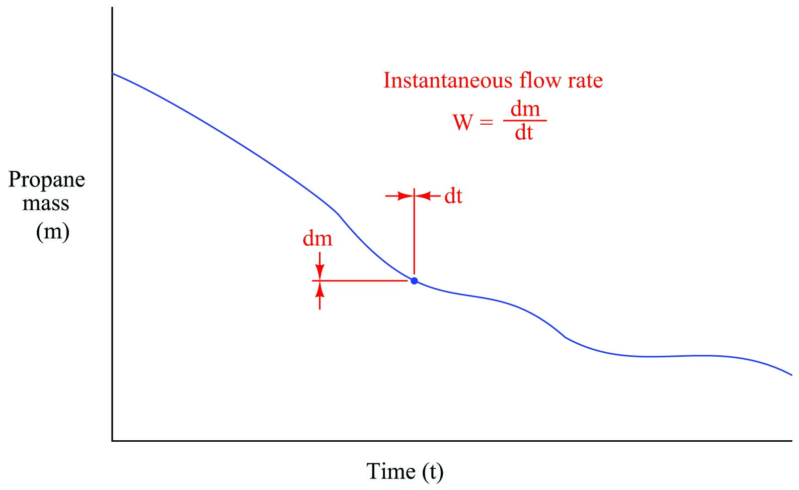
\[W = {dm \over dt} = \hbox{Instantaneous mass flow rate}\]
Where,
\(W\) = Instantaneous mass flow rate at a given time (kilograms per minute)
\(dm\) = Mass differential at a single point in time (kilograms)
\(dt\) = Time differential at a single point in time (minutes)
Flow is calculated just the same as before: a quotient of mass and time differences, except here the differences are infinitesimal in magnitude. The unit of flow measurement reflects this process of division, just as before, with mass flow rate expressed in units of kilograms per minute. Also, just as before, the rate of flow is graphically represented by the slope of the graph: steeply-sloped points on the graph represent moments of high flow rate, while shallow-sloped points on the graph represent moments of low flow rate.
Such a ratio of differential quantities is called a derivative in calculus. Derivatives – especially time-based derivatives such as flow rate – find many applications in instrumentation as well as the general sciences. Some of the most common time-based derivative functions include the relationships between position (\(x\)), velocity (\(v\)), and acceleration (\(a\)).
Velocity (\(v\)) is the rate at which an object changes position over time. Since position is typically denoted by the variable \(x\) and time by the variable \(t\), the derivative of position with respect to time may be written as such:
\[v = {dx \over dt} \hskip 50pt [\hbox{meters/second}] = {[\hbox{meters}] \over [\hbox{seconds}]}\]
The metric units of measurement6 for velocity (meters per second, miles per hour, etc.) betray this process of division: a differential of position (meters) divided by a differential of time (second).
Acceleration (\(a\)) is the rate at which an object changes velocity over time. Thus, we may express acceleration as the time-derivative of velocity, just as velocity was expressed as the time-derivative of position:
\[a = {dv \over dt} \hskip 50pt [\hbox{meters/second}^2] = {[\hbox{meters/second}] \over [\hbox{seconds}]}\]
We may even express acceleration as a function of position (\(x\)), since it is the rate of change of the rate of change in position over time. This is known as a second derivative, since it is applying the process of “differentiation” twice:
\[a = {d \over dt} \left({dx \over dt}\right) = {d^2 x \over dt^2} \hskip 50pt [\hbox{meters/second}^2] = {[\hbox{meters}] \over [\hbox{seconds}^2]}\]
As with velocity, the units of measurement for acceleration (meters per second squared, or alternatively meters per second per second) suggest a compounded quotient.
It is also possible to express rates of change between different variables not involving time. A common example in the engineering realm is the concept of gain, generally defined as the ratio of output change to input change. An electronic amplifier, for example, with an input signal of 2 volts (peak-to-peak) and an output signal of 8.6 volts (peak-to-peak), would be said to have a gain of 4.3, since the change in output measured in peak-to-peak volts is 4.3 times larger than the corresponding change in input voltage:
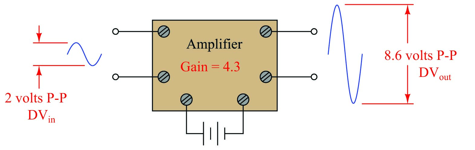
This gain may be expressed as a quotient of differences (\(\Delta V_{out} \over \Delta V_{in}\)), or it may be expressed as a derivative instead:
\[\hbox{Gain} = {dV_{out} \over dV_{in}}\]
If the amplifier’s behavior is perfectly linear, there will be no difference between gain calculated using differences and gain calculated using differentials (the derivative), since the average slope of a straight line is the same as the instantaneous slope at any point along that line. If, however, the amplifier does not behave in a perfectly linear fashion, gain calculated from large changes in voltage (\(\Delta V_{out} \over \Delta V_{in}\)) will not be the same as gain calculated from infinitesimal changes at different points along the amplifier’s operating voltage range.

Whoever wrote this calculus tutor is brilliant!!! Thank you