 Facebook
 Google
 GitHub
 Linkedin
The Concept of Integration
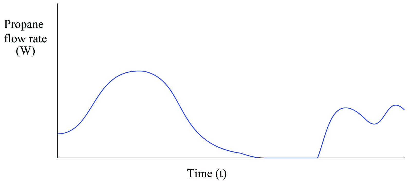
Suppose we wished to measure the consumption of propane over time for a large propane storage tank supplying a building with heating fuel, because the tank lacked a level indicator to show how much fuel was left at any given time. The flow rate is sufficiently large, and the task sufficiently important, to justify the installation of a mass flowmeter, which registers flow rate at an indicator inside the building:
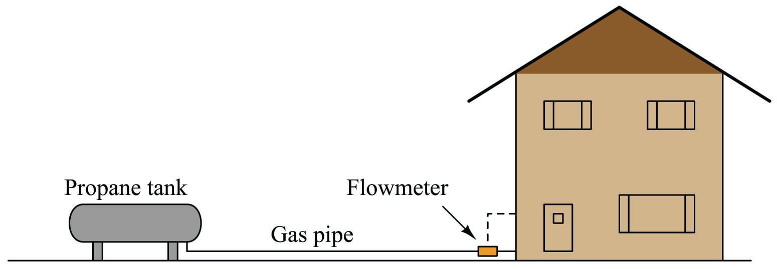
By measuring true mass flow rate, it should be possible to indirectly measure how much propane has been used at any time following the most recent filling of the tank. For example, if the mass flow rate of propane out of the tank happened to be a constant 5 kilograms per hour for 30 hours straight, it would be a simple matter of multiplication to calculate the consumed mass:
\[\left(5 \hbox{ kg} \over \hbox{hr} \right) \left(30 \hbox{ hrs} \over 1 \right) = 150 \hbox{ kg of propane consumed}\]
Expressing this mathematically as a function of differences in mass and differences in time, we may write the following equation:
\[\Delta m = \overline{W} \> \Delta t\]
Where,
\(\overline{W}\) = Average mass flow rate within the time period (kilograms per hour)
\(\Delta m\) = Mass difference over time period (kilograms)
\(\Delta t\) = Time period of flow measurement sample (hours)
It is easy to see how this is just a variation of the quotient-of-differences equation used previously in this chapter to define mass flow rate:
\[\overline{W} = {\Delta m \over \Delta t} = \hbox{Average mass flow rate}\]
Inferring mass flow rate from changes in mass over time periods is a process of division. Inferring changes in mass from flow rate over time periods is a process of multiplication. The units of measurement used to express each of the variables makes this quite clear.
As we learned previously, the process of differentiation is really just a matter of determining the slope of a graph. A graph of propane fuel mass (\(m\)) plotted over discrete points in time (\(t\)) has a slope corresponding to mass flow rate (\(W = {\Delta m \over \Delta t}\)). Here, we are attempting to do the opposite: the data reported by the sensing instrument is propane mass flow rate (\(W\)), and our goal is to determine total mass lost (\(\Delta m\)) as the propane is consumed from the storage tank over a period of time (\(\Delta t\)). This operation is fundamentally distinct from differentiation, which means its graphical interpretation will not be the same. Instead of calculating the slope of the graph, we will have to do something else.
Using the previous example of the propane flowmeter sensing a constant mass flow rate (\(W\)) of 5 kilograms of propane per hour for 30 hours (for a total consumption of 150 kilograms), we may plot a trend graph showing flow rate (vertical) as a function of time (horizontal). We know the consumed propane quantity is the simple product (multiplication) of constant flow rate and time, which relates to the geometric area enclosed by the graph, since the area of any rectangle is height times width:
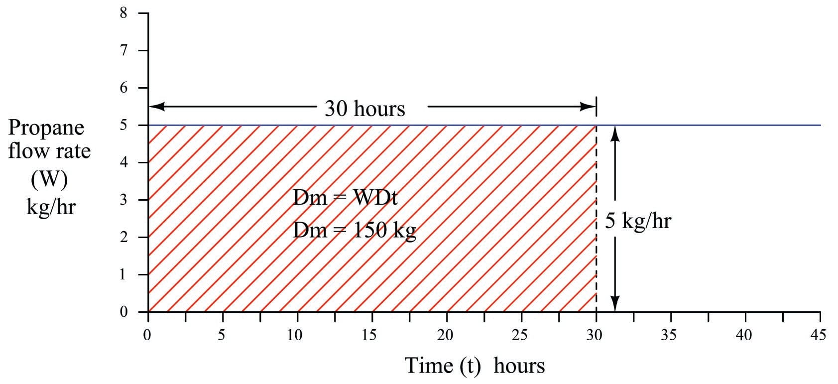
To summarize: the height of this graph represents the rate at which propane exits the storage tank, the width of the graph represents the length of time propane has been consumed from the storage tank, and the geometric area enclosed by these two boundaries represents the total mass of propane consumed during that time.
The task of inferring lost mass over time becomes more complicated if the propane flow rate is not constant over time. Consider the following graph, showing periods of increased and decreased flow rate due to different gas-fired appliances turning on and off inside the building:
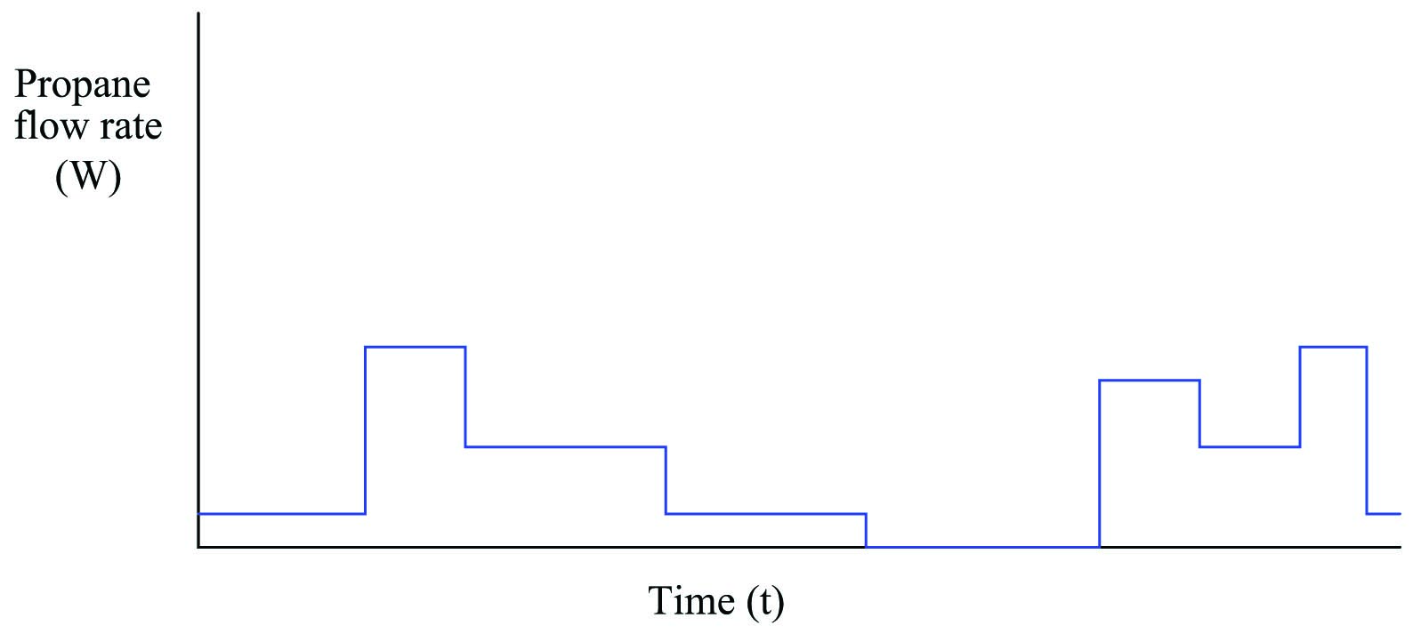
Here, the propane gas flow rate does not stay constant throughout the entire time interval covered by the graph. This graph is obviously more challenging to analyze than the previous example where the propane flow rate was constant. From that previous example, though, we have learned that the geometric area enclosed by the boundaries of the graph’s height (flow rate) and width (time duration) has physical meaning, representing the total quantity of propane passed through the flowmeter. Despite the fact that the graph’s area is now more complex to calculate, the basic principle remains the same as before: the enclosed area represents the amount of propane consumed.
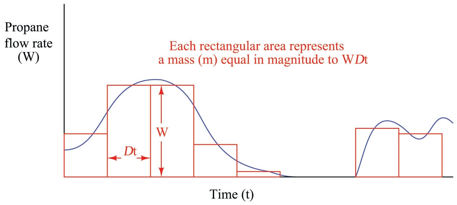
In order to accurately calculate the amount of propane mass consumed by the building over time, we must treat each period of constant flow as its own propane quantity, calculating the mass lost during each period, then summing those mass differences to arrive at a total mass loss for the entire time interval covered by the graph. Since we know the difference (loss) in mass over a time period is equal to the average flow rate for that period multiplied by the period’s duration (\(\Delta m = W \> \Delta t\)), we may calculate each period’s mass as an area underneath the graph line, each rectangular area being equal to height (\(W\)) times width (\(\Delta t\)):
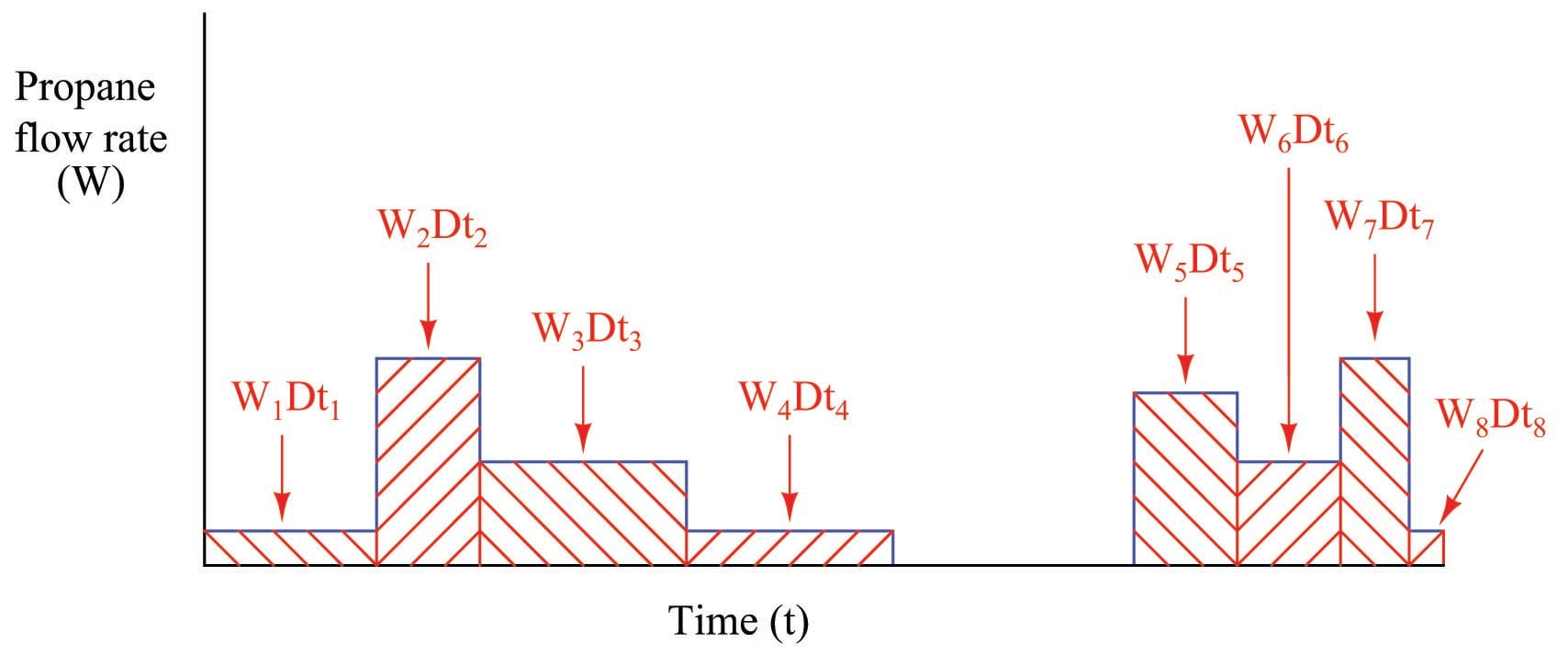
Each rectangular area underneath the flow line on the graph (\(W_n \Delta t_n\)) represents a quantity of propane gas consumed during that time period. To find the total amount of propane consumed in the time represented by the entire graph, we must sum these mass quantities together:
\[\Delta m = (W_1 \Delta t_1) + (W_2 \Delta t_2) + (W_3 \Delta t_3) + (W_4 \Delta t_4) + (W_5 \Delta t_5) + (W_6 \Delta t_6) + (W_7 \Delta t_7) + (W_8 \Delta t_8)\]
A “shorthand” notation for this sum uses the capital Greek letter sigma to represent a series of repeated products (multiplication) of mass flow and time periods for the eight rectangular areas enclosed by the graph:
\[\Delta m = \sum_{n=1}^8 W_n \> \Delta t_n\]
While \(W_n \Delta t_n\) represents the area of just one of the rectangular periods, \(\sum_{n=1}^8 W_n \Delta t_n\) represents the total combined areas, which in this example represents the total mass of propane consumed over the eight time periods shown on the graph.
The task of inferring total propane mass consumed over time becomes even more complicated if the flow does not vary in stair-step fashion as it did in the previous example. Suppose the building were equipped with throttling gas appliances instead of on/off gas appliances, thus creating a continuously variable flow rate demand over time. A typical flow rate graph might look something like this:
The physics of gas flow and gas mass over time has not changed: total propane mass consumed over time will still be the area enclosed beneath the flow curve. The only difference between this example and the two previous examples is the complexity of actually calculating that enclosed area.
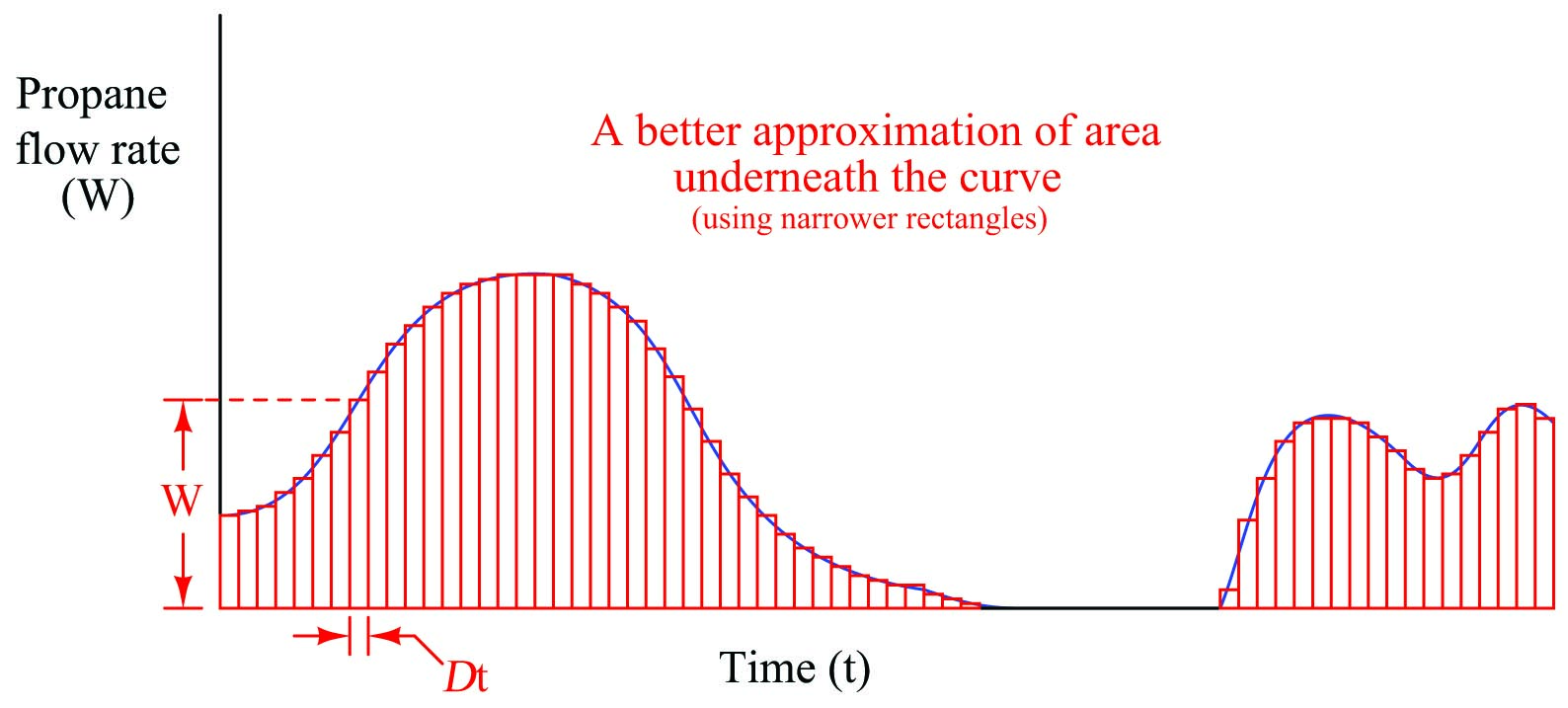
We can, however, approximate the area underneath this curve by overlaying a series of rectangles, the area of each rectangle being height (\(W\)) times width (\(\Delta t\)):
It should be intuitively obvious that this strategy of approximating the area underneath a curve improves with the number of rectangles used. Each rectangle still has an area \(W \Delta t\), but since the \(\Delta t\) periods are shorter, it is easier to fit the rectangles to the curve of the graph. The summation of a series of rectangular areas intended to approximate the area enclosed by a graphed function is commonly referred to as a Riemann Sum in honor of the mathematician Bernhard Riemann:
Taking this idea to its ultimate realization, we could imagine a super-computer sampling mass flow rates at an infinite speed, then calculating the rectangular area covered by each flow rate (\(W\)) times each infinitesimal increment of time (\(dt\)). With time increments of negligible width, the “approximation” of area underneath the graph found by the sum of all these rectangles would be perfect – indeed, it would not be an approximation at all, but rather an exact match:
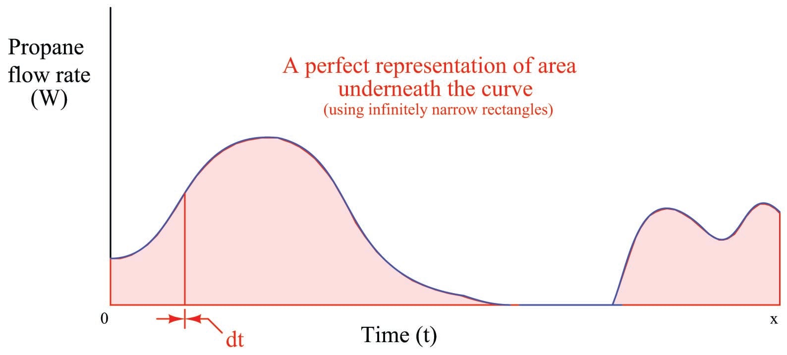
If we represent infinitesimal time increments using the notation “\(dt\)” as opposed to the notation “\(\Delta t\)” used to represent discrete time periods, we must also use different notation to represent the mathematical sum of those quantities. Thus, we will replace the “sigma” symbol (\(\sum\)) used for summation and replace it with the integral symbol (\(\int\)), which means a continuous summation of infinitesimal quantities:
\[\Delta m = \sum_{n=0}^x W \> \Delta t_n \hskip 30pt \hbox{Summing discrete quantities of } W \Delta t\]
\[\Delta m = \int_0^x W \> dt \hskip 30pt \hbox{Summing continuous quantities of } W \> dt\]
This last equation tells us the total change in mass (\(\Delta m\)) from time 0 to time \(x\) is equal to the continuous sum of mass quantities found by multiplying mass flow rate measurements (\(W\)) over corresponding increments of time (\(dt\)). We refer to this summation of infinitesimal quantities as integration in calculus. Graphically, the integral of a function is the geometric area enclosed by the function over a specified interval.
An important detail to note is that this process of integration (multiplying flow rates by infinitesimal time increments, then summing those products) only tells us how much propane mass was consumed – it does not tell us how much propane remains in the tank, which was the purpose of installing the mass flowmeter and performing all this math! The integral of mass flow and time (\(\int W \> dt\)) will always be a negative quantity in this example, because a flow of propane gas out of the tank represents a loss of propane mass within the tank. In order to calculate the amount of propane mass left in the tank, we would need to know the initial value of propane in the tank before any of it flowed to the building, then we would add this initial mass quantity (\(m_0\)) to the negative mass loss calculated by integration.
Thus, we would mathematically express the propane mass inside the tank at time \(x\) as such:
\[m_x = \int_0^x W \> dt + m_0\]
This initial value must always be considered in problems of integration if we attempt to absolutely define some integral quantity. Otherwise, all the integral will yield is a relative quantity (how much something has changed over an interval).
The problem of initial values is very easy to relate to common experience. Consider the odometer indication in an automobile. This is an example of an integral function, the distance traveled (\(x\)) being the time-integral of speed (or velocity, \(v\)):
\[\Delta x = \int v \> dt\]
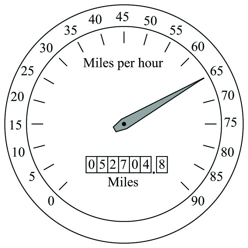
Although the odometer does accumulate to larger and larger values as you drive the automobile, its indication does not necessarily tell me how many miles you have driven it. If, for example, you purchased the automobile with 32411.6 miles on the odometer, its current indication of 52704.8 miles means that you have driven it 20293.2 miles. The automobile’s total distance traveled since manufacture is equal to the distance you have accumulated while driving it (\(\int v \> dt\)) plus the initial mileage accumulated at the time you took ownership of it (\(x_0\)):
\[x_{total} = \int v \> dt + x_0\]

Nice text book