 Facebook
 Google
 GitHub
 Linkedin
The s Variable: Euler’s Relation and Phasor Expressions of Waveforms
The magnitude of waves over time is expressed with a combined real and imaginary term
The s variable, this combination of a real and imaginary component of a vector, simplifies the mathematical expression used to predict systems like volts, amps, and even the physical motion of real systems over time.
A powerful mathematical concept useful for analyzing practically any physical system – electrical circuits included – is something called the \(s\) variable. The \(s\) variable is closely related to Euler’s Relation and phasor expressions of waveforms, which is why a discussion of it is included here.
Meaning of the \(s\) Variable
As we saw previously, Euler’s Relation allows us to express rotating phasors as imaginary exponents of \(e\). For example, \(Ae^{j \theta}\) represents a phasor of length \(A\) at an angle of \(\theta\) radians. \(Ae^{j \omega t}\) represents a phasor of length \(A\) rotating at a velocity of \(\omega\) radians per second at a particular instant in time \(t\). This happens to be an incredibly useful mathematical “trick” for representing sinusoidal waves in physical systems. For example, if we wished to mathematically express a sinusoidal AC voltage as a function of time with a peak voltage value of 10 volts and a frequency of 60 hertz (377 radians per second, since \(\omega = 2 \pi f\)), we could do so like this:
\[V(t) = 10 e^{j377t}\]
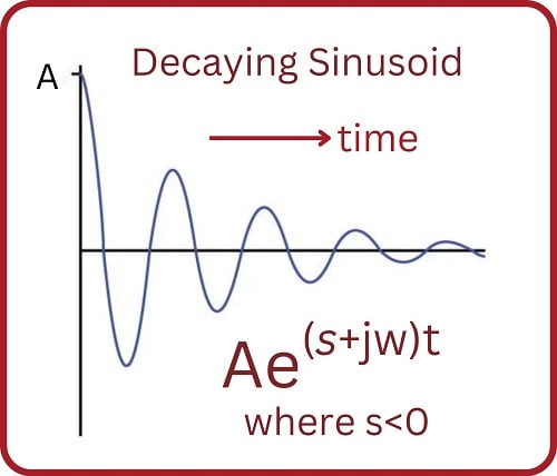
Exponential functions aren’t just useful for expressing sinusoidal waves, however. They also work well for expressing rates of growth and decay, as is the case with RC and L/R time-delay circuits where exponential functions describe the charging and discharging of capacitors and inductors. Here, the exponent is a real number rather than an imaginary number: the expression \(e^{-t / \tau}\) approaching zero as time (\(t\)) increases. The Greek letter “tau” (\(\tau\)) represents the time constant of the circuit, which for capacitive circuits is the product of \(R\) and \(C\), and for inductive circuits is the quotient of \(L\) and \(R\). For example, if we wished to mathematically express the decaying voltage across a 33 \(\mu\)F capacitor initially charged to 10 volts as it dissipates its stored energy through a 27 k\(\Omega\) resistor (the circuit having a time constant of 0.891 seconds, since \(\tau = RC\)), we could do so like this:
\[V(t) = 10 e^{-(t / 0.891)}\]
The sign of the exponential term here is very important: in this example we see it is a negative number. This tells us the function decays (approaches zero) over time, since larger positive values of \(t\) result in larger negative values of \(t / \tau\) (recall from algebra that a negative exponent is the equivalent of reciprocating the expression, so that \(e^{-x} = {1 \over {e^x}}\)). If the exponent were a real positive number, it would represent some quantity growing exponentially over time. If the exponent were zero, it would represent a constant quantity. We expect a discharging resistor-capacitor circuit to exhibit decaying voltage and current values, and so the negative exponent sign shown here makes sense.
If imaginary exponents of \(e\) represent phasors, and real exponents of \(e\) represent growth or decay, then a complex exponent of \(e\) (having both real and imaginary parts) must represent a phasor that grows or decays in magnitude over time. Engineers use the lower-case Greek letter “omega” (\(\omega\)) along with the imaginary operator \(j\) to represent the imaginary portion, and the lower-case Greek letter “sigma” (\(\sigma\)) to represent the real portion. For example, if we wished to mathematically express a sine wave AC voltage with a frequency of 60 hertz (377 radians per second) and an amplitude beginning at 10 volts but decaying with a time constant (\(\tau\)) of 25 milliseconds (\(\sigma = 1 / \tau\) = 40 time constants per second), we could do so like this:
\[V(t) = 10 e^{-40t + j377t}\]
We may factor time from the exponential terms in this expression, since \(t\) appears both in the real and imaginary parts:
\[V(t) = 10 e^{(-40 + j377)t}\]
With \(t\) factored out, the remaining terms \(-40 + j377\) completely describe the sinusoidal wave’s characteristics. The wave’s decay rate is described by the real term (\(\sigma = -40\) time constants per second), while the wave’s phase is described by the imaginary term (\(j \omega = 377\) radians per second). Engineers use a single variable \(s\) to represent the complex quantity \(\sigma + j\omega\), such that any growing or decaying sinusoid may be expressed very succinctly as follows:
\[Ae^{st} = Ae^{(\sigma + j\omega)t} = Ae^{\sigma t} e^{j \omega t}\]
Where,
\(A\) = Initial amplitude of the sinusoid (e.g. volts, amps) at time \(t = 0\) (arbitrary units)
\(s\) = Complex growth/decay rate and frequency (sec\(^{-1}\))
\(\sigma\) = \(1 \over \tau\) = Real growth/decay rate (time constants per second, or sec\(^{-1}\))
\(j \omega\) = Imaginary frequency (radians per second, or sec\(^{-1}\))
\(t\) = Time (seconds)
Separating the expression \(Ae^{\sigma t} e^{j \omega t}\) into three parts – \(A\), \(e^{\sigma t}\), and \(e^{j \omega t}\) – we get a complete description of a rotating phasor:
\(A\) = Initial amplitude of the phasor (\(t = 0\))
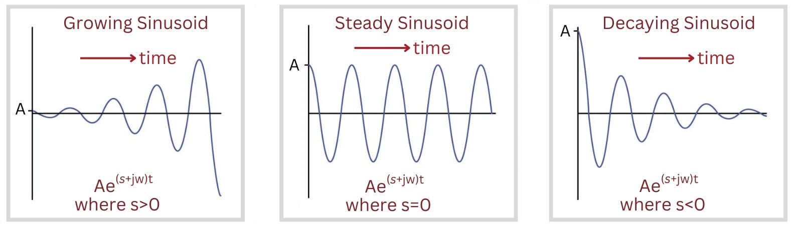
\(e^{\sigma t}\) = How much the phasor’s magnitude has grown (\(\sigma > 0\)) or decayed (\(\sigma < 0\)) at time \(t\)
\(e^{j \omega t}\) = Unit phasor (length = 1) at time \(t\)
If we set \(\omega\) at some constant value and experiment with different values of \(\sigma\), we can see the effect \(\sigma\) has on the shape of the wave over time:
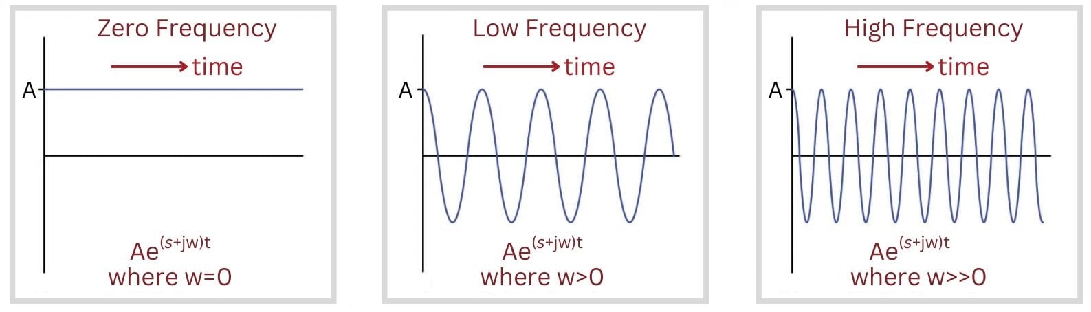
If we set \(\sigma\) at zero and experiment with different values of \(\omega\), we can see the effect \(\omega\) has on the shape of the wave over time:
As we will soon see, characterizing a sinusoidal response using the complex variable \(s\) allows us to mathematically describe a great many things. Not only may we describe voltage waveforms using \(s\) as shown in these simple examples, but we may also describe the response of entire physical systems including electrical circuits, machines, feedback control systems, and even chemical reactions. In fact, it is possible to map the essential characteristics of any linear system in terms of how exponentially growing, decaying, or steady sinusoidal waves affect it, and that mapping takes the form of mathematical functions of \(s\).
When engineers or technicians speak of a resonant system, they mean a circuit containing inductive and capacitive elements tending to sustain oscillations of a particular frequency (\(\omega\)). A lossless resonant system (e.g. a superconducting tank circuit, a frictionless pendulum) may be expressed by setting the real portion of \(s\) equal to zero (\(\sigma = 0\) ; no growth or decay) and letting the imaginary portion represent the resonant frequency (\(j \omega = j 2 \pi f\)). Real-life resonant systems inevitably dissipate some energy, and so a real resonant system’s expression will have both an imaginary portion to describe resonant frequency and a negative real portion to describe the oscillation’s rate of decay over time.
Systems exhibiting a positive \(\sigma\) value are especially interesting because they represent instability: unrestrained oscillatory growth over time. A feedback control loop with excessive gain programmed into the loop controller is a simple example of a system where \(\sigma > 1\). This situation, of course, is highly undesirable for any control system where the goal is to maintain the process variable at a steady setpoint.
Impedance Expressed Using the \(s\) Variable
Previously, we saw how the impedance of inductors and capacitors could be calculated using \(j \omega\) to represent the frequency of the applied signal. Doing so greatly simplified the mathematics by eliminating the need to manipulate trigonometric functions such as sine and cosine. Here, we will discover that \(s\) works just as nicely for the same task, with the added benefit of showing how inductors and capacitors react to exponentially growing or decaying signals.
First, let’s begin with capacitors. We know that voltage across a capacitor and current “through” a capacitor are related as follows:
\[I = C {dV \over dt}\]
Next, we substitute an expression for voltage in terms of \(s\) and then use calculus to differentiate it with respect to time:
\[I = C {d \over dt}\left(e^{st}\right)\]
\[I = sC e^{st}\]
The ratio of \(V \over I\) (the definition of impedance) will then be:
\[Z_C = {V \over I} = {e^{st} \over sC e^{st}}\]
\[Z_C = {1 \over sC}\]
Instead of the common scalar expression for capacitive impedance (\(Z_C = {1 \over {2 \pi f C}}\)) which only tells us the magnitude of the impedance (in ohms) but not the phase shift, we have a complex expression for capacitive impedance (\(Z_C = {1 \over sC}\)) describing magnitude, phase shift, and its reaction to the growth or decay of the signal.
Likewise, we may do the same for inductors. Recall that voltage across an inductor and current through an inductor are related as follows:
\[V = L {dI \over dt}\]
Substituting an expression for current in terms of \(s\) and using calculus to differentiate it with respect to time:
\[V = L {d \over dt}\left(e^{st}\right)\]
\[V = sL e^{st}\]
The ratio of \(V \over I\) (the definition of impedance) will then be:
\[Z_L = {V \over I} = {sL e^{st} \over e^{st}}\]
\[Z_L = sL\]
As with capacitors, we now have a complex expression for inductive impedance describing magnitude, phase shift, and its reaction to signal growth or decay (\(Z_L = sL\)) instead of merely having a scalar expression for inductive impedance (\(Z_L = 2 \pi f L\)).
Resistors directly oppose current by dropping voltage, with no regard to rates of change. Therefore, there are no derivatives in the relationship between voltage across a resistor and current through a resistor:
\[V = IR\]
If we substitute \(e^{st}\) for current into this formula, we will see that voltage must equal \(Re^{st}\). Solving for the ratio of voltage over current to define impedance:
\[Z_R = {V \over I} = {Re^{st} \over e^{st}}\]
\[Z_R = R\]
Not surprisingly, all traces of \(s\) cancel out for a pure resistor: its impedance is exactly equal to its DC resistance.
In summary:
| Inductive impedance (\(Z_L\)) | Capacitive impedance (\(Z_C\)) | Resistive impedance (\(Z_R\)) |
|---|---|---|
| \(sL\) | \(1 / sC\) | \(R\) |
Now let’s explore these definitions of impedance using real numerical values. First, let’s consider a 22 \(\mu\)F capacitor exposed to a steady AC signal with a frequency of 500 Hz. Since the signal in this case is steady (neither growing nor decaying in magnitude), the value of \(\sigma\) will be equal to zero. \(\omega\) is equal to \(2 \pi f\), and so a frequency of 500 Hz is equal to 3141.6 radians per second. Calculating impedance is as simple as substituting these values for \(s\) and computing \(1 / sC\):
\[Z_C = {1 \over sC} = {1 \over (\sigma + j \omega) C}\]
\[Z_C = {1 \over (0 + j 3141.6 \hbox{ sec}^{-1}) (22 \times 10^{-6} \hbox{ F})}\]
\[Z_C = {1 \over j 0.0691}\]
\[Z_C = {-j \over 0.0691}\]
\[Z_C = 0 - j 14.469 \> \Omega \hspace{10pt} \hbox{(rectangular notation)}\]
\[Z_C = 14.469 \> \Omega \> \angle -90^{o} \hspace{10pt} \hbox{(polar notation)}\]
Thus, the impedance of this capacitor will be 14.469 ohms at a phase angle of \(-90^{o}\). The purely imaginary nature of this impedance (its orthogonal phase shift between voltage and current) tells us there is no net power dissipated by the capacitor. Rather, the capacitor spends its time alternately absorbing and releasing energy to and from the circuit.
Next, we will consider the case of a 150 mH inductor exposed to an exponentially rising DC signal with a time constant (\(\tau\)) of 5 seconds. 5 seconds per time constant (\(\tau\)) is equal to 0.2 time constants per second (\(\sigma\)). Since the signal in this case is DC and not AC, the value of \(\omega\) will be equal to zero. Calculating impedance, once again, is as simple as substituting these values for \(s\) and computing \(sL\):
\[Z_L = sL = (\sigma + j \omega)L\]
\[Z_L = (0.2 + j 0 \hbox{ sec}^{-1})(150 \times 10^{-3} \hbox{ H})\]
\[Z_L = 0.03 + j 0 \> \Omega \hspace{10pt} \hbox{(rectangular notation)}\]
\[Z_L = 0.03 \> \Omega \> \angle 0^{o} \hspace{10pt} \hbox{(polar notation)}\]
Thus, the impedance of this inductor will be 0.03 ohms at a phase angle of 0\(^{o}\). The purely real nature of this impedance (i.e. no phase shift between voltage and current) tells us energy will be continually absorbed by the inductor, and for this reason it will be seen by the rest of the circuit as though it were a resistor dissipating energy for however long the signal continues to exponentially grow.
A phase shift of 0 degrees for a reactive component such as an inductor may come as a surprise to students accustomed to thinking of inductive impedances always having 90 degree phase shifts! However, the application of the complex variable \(s\) to impedance mathematically demonstrates we can indeed have conditions of no phase shift given just the right circumstances. This makes conceptual sense as well if we consider how inductors store energy: if the current through an inductor increases exponentially over time, never reversing direction, it means the inductor’s magnetic field will always be growing and therefore absorbing more energy from the rest of the circuit.
We see something even more interesting happen when we subject a reactive component to a decaying DC signal. Take for example a 33,000 \(\mu\)F capacitor exposed to a decaying DC signal with a time constant of 65 milliseconds. 65 milliseconds per time constant (\(\tau\)) is equal to 15.38 time constants per second (\(\sigma\)). Once again \(\omega\) will be zero because this is a non-oscillating signal. Calculating capacitive impedance:
\[Z_C = {1 \over sC} = {1 \over (\sigma + j \omega) C}\]
\[Z_C = {1 \over (-15.38 + j 0 \hbox{ sec}^{-1}) (33000 \times 10^{-6} \hbox{ F})}\]
\[Z_C = {1 \over -0.508}\]
\[Z_C = -1.970 + j 0 \> \Omega \hspace{10pt} \hbox{(rectangular notation)}\]
\[Z_C = 1.970 \> \Omega \> \angle 180^{o} \hspace{10pt} \hbox{(polar notation)}\]
A negative real impedance figure represents a phase shift of 180\(^{o}\) between voltage and current. Once again, this may surprise students of electronics who are accustomed to thinking of capacitive impedances always having phase shifts of \(-90\) degrees. What a 180 degree phase shift means is the direction of current with respect to voltage polarity has the capacitor functioning as an energy source rather than as a load. If we consider what happens to a capacitor when it discharges, the 180 degree phase shift makes sense: current flowing in this direction depletes the capacitor’s plates of stored charge, which means the electric field within the capacitor weakens over time as it releases that energy to the rest of the circuit.
