 Facebook
 Google
 GitHub
 Linkedin
Transfer Function Analysis
Predicting time-response for systems can be difficult without transfer functions
Transfer functions express how the output of a machine or circuit will respond, based on the poles and zeroes of the system and the input signal, which may be an applied force or a voltage waveform.
An extremely important topic in engineering is that of transfer functions. Simply defined, a transfer function is the ratio of output to input for any physical system, usually with both the output and input being mathematical functions of \(s\). In other words, we express both the output of a system and the corresponding input of that system in terms of exponentially growing/decaying sinusoidal waves and then solve for the ratio of those two expressions.
Unfortunately, the teaching of transfer functions and their relation to real-world phenomena is often obfuscated by a heavy emphasis on mathematics. The intent of this section is to introduce this concept in a way that is very “gentle” and continually referenced to real-world applications. If I can do anything to help lift the veil of mystery surrounding concepts such as transfer functions, the \(s\) variable, and pole-zero plots, then technicians as well as engineers will be able to appreciate the power of this analytical technique and be able to exchange more ideas in the same “language”.
What is a Transfer Function?
A simple example of a transfer function is the gain of an electronic amplifier. As all students of electronics learn, “gain” is the ratio of output signal to input signal for a circuit. Beginning students learn to represent circuit gains as scalar values (e.g. “The amplifier has a voltage gain of 24”), first as plain ratios and later as decibel figures (e.g. “The amplifier has a voltage gain of 27.6 dB”). One limitation of this approach is that it oversimplifies the situation when the gain of the circuit in question varies with the frequency and/or the growth/decay rate of the signal, which is quite often the case. If we take the engineering approach of expressing output and input signals as functions of \(s\), we obtain a more complete picture of that circuit’s behavior over a wide range of conditions.
Another simple example of a transfer function is what we have just seen in this book: the impedance of a reactive electrical component such as a capacitor or an inductor. Here, the ratio in question is between voltage and current. If we consider current through the component to be the “input” signal and voltage across the component to be the “output” signal – both expressed in terms of \(s\) – then impedance \(Z(s) = {V(s) \over I(s)}\) is the transfer function for that component. This raises an important point about transfer functions: what we define as the “input” and the “output” of the system is quite arbitrary, so long as there is an actual relationship between the two signals.
Poles and Zeros of Transfer Function Circuits
If we write generalized output/input transfer functions of \(s\) for an AC circuit, we may mathematically analyze that transfer function to gain insight into the behavior and characteristics of that circuit. Features of transfer functions of interest to us include:
- Zeros: any value(s) of \(s\) resulting in a zero value for the transfer function (i.e. zero gain)
- Poles: any value(s) of \(s\) resulting in an infinite value for the transfer function (i.e. maximum gain)
An AC circuit’s zeros tell us where the circuit is unresponsive to input stimuli. An AC circuit’s poles tell us where the circuit is able to generate an output signal with no input stimulus (i.e. its natural or un-driven mode(s) of response).
In order to clearly understand the concept of transfer functions, practical examples are very helpful. Here we will explore some very simple AC circuits in order to grasp what transfer functions are and how they benefit system analysis.
LR Low Pass Filter Circuit
First, let’s begin with a simple low-pass filter circuit comprised of an inductor and a resistor connected in series:
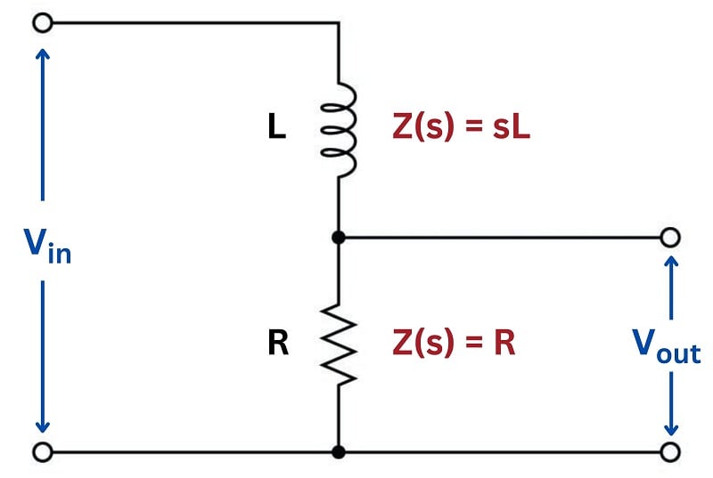
The impedance of each component as a function of \(s\) is shown in the diagram: the inductor’s impedance is \(sL\) while the resistor’s impedance is simply \(R\). It should be clear to any student of electronics that these two components will function as a voltage divider, with the output voltage being some fraction of the input voltage.
Low Pass Filter Transfer Function
Knowing the circuit impedance, we may write a transfer function for this circuit based on the voltage divider formula, which tells us the ratio of output voltage to input voltage is the same as the ratio of output impedance to total impedance:
\[\hbox{Transfer function} = {V_{out}(s) \over V_{in}(s)}\]
\[{R \over {R + sL}} = {R \over {R + (\sigma + j \omega) L}}\]
This transfer function allows us to calculate the “gain” of the system for any given value of \(s\), which brings us to the next step of our analysis. At this point we will ask ourselves three questions:
- How does this system respond when \(s = 0\)?
- What value(s) of \(s\) make the transfer function approach a value of zero?
- What value(s) of \(s\) make the transfer function approach a value of infinity?
The first of these questions refers to a condition where we apply a steady DC signal to the input of the system. If \(s = 0\) then both \(\sigma\) and \(\omega\) must each be equal to zero. A value of zero for \(\sigma\) means the signal is neither growing nor decaying over time, but remains at some unchanging value. A value of zero for \(\omega\) means the signal is not oscillating. These two conditions can only refer to a steady DC signal applied to the circuit. Substituting zero for \(s\) we get:
\[{R \over {R + 0 L}}\]
\[{R \over R} = 1\]
Therefore the transfer function of this circuit is unity (1) under DC conditions. This is precisely what we would expect given an inductor connected in series with a resistor, with output voltage taken across the resistor. If there is no change in the applied signal, then the inductor’s magnetic field will be unchanging as well, which means it will drop zero voltage (assuming a pure inductor with no wire resistance) leaving the entire input voltage dropped across the resistor.
The second question refers to a condition where the output signal of this circuit is zero. Any values of \(s\) resulting in zero output from the system are called the zeros of the transfer function. Examining the transfer function for this particular low-pass LR filter circuit, we see that this can only be true if \(s\) becomes infinitely large, because \(s\) is located in the denominator of the fraction:
\[{R \over {R \pm \infty L}} = 0\]
This is consistent with the behavior of a low-pass filter: as frequency (\(\omega\)) increases, the filter’s output signal diminishes. The transfer function doesn’t just tell us how this circuit will respond to change in frequency, however – it also tells us how the circuit will respond to growing or decaying signals too. Here, we see that infinitely large \(\sigma\) values also result in zero output: the inductor, which tends to oppose any current exhibiting a high rate of change, doesn’t allow much voltage to develop across the resistor if the input signal is growing or decaying very rapidly.
The third question refers to a condition where either the transfer function’s numerator approaches infinity or its denominator approaches zero. Any values of \(s\) having this result are called the poles of the transfer function. Since the numerator in this particular case is a constant (\(R\)), only a denominator value of zero could cause the transfer function to reach infinity:
\[{R \over {R + sL}} = \infty \hbox{ only if } R + sL = 0\]
If the necessary condition for a “pole” is that \(R + sL = 0\), then we may solve for \(s\) as follows:
\[R + sL = 0\]
\[sL = -R\]
\[s = -{R \over L}\]
Thus, this transfer function for this simple low-pass filter circuit has one pole located at \(s = - R / L\). Since both \(R\) and \(L\) are real numbers (not imaginary) with positive values, then the value of \(s\) for the pole must be a real number with a negative value. In other words, the solution for \(s\) at this pole is all \(\sigma\) and no \(\omega\): this refers to an exponentially decaying DC signal.
It is important at this point to consider what this “pole” condition means in real life. The notion that a circuit is able to produce an output signal with zero input signal may sound absurd, but it makes sense if the circuit in question has the ability to store and release energy. In this particular circuit, the inductor is the energy-storing component, and it is able to produce a voltage drop across the resistor with zero input voltage in its “discharging” mode.
An illustration helps make this clear. If the “pole” condition is such that \(V_{in}(s) = 0\), we may show this by short-circuiting the input of our filter circuit to ensure a zero-input condition:
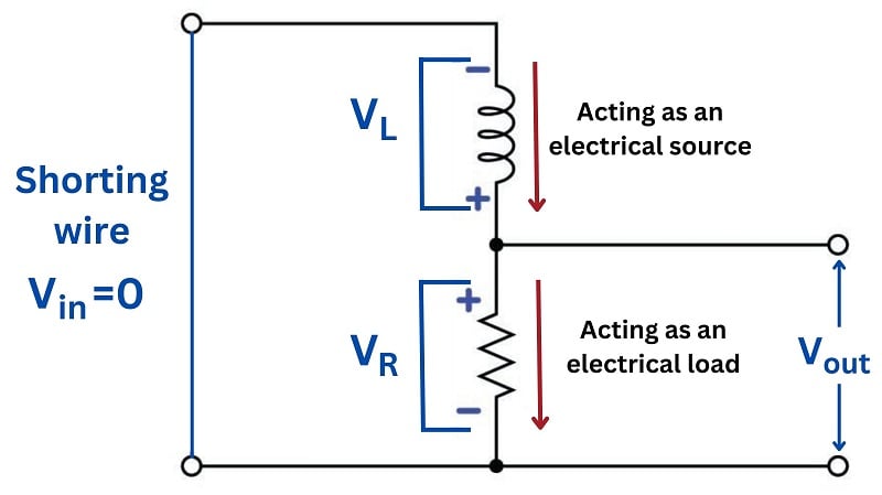
Assuming the inductor has been “charged” with energy previous to the short-circuiting of the input, an output voltage will surely develop across the resistor as the inductor discharges. In other words, the inductor behaves as an electrical source while the resistor behaves as an electrical load: connected in series they must of course share the same current, but their respective voltages are equal in magnitude and opposing in polarity in accordance with Kirchhoff’s Voltage Law. Furthermore, the value of \(s\) in this “pole” condition tells us exactly how rapidly the output signal will decay: it will do so at a rate \(\sigma = -R / L\). Recall that the growth/decay term of the \(s\) variable the reciprocal of the system’s time constant (\(\sigma = 1 / \tau\)). Therefore, a \(\sigma\) value of \(R / L\) is equivalent to a time constant of \(L / R\), which as all beginning students of electronics learn is how we calculate the time constant for a simple inductor-resistor circuit.
Transfer functions are easier to understand when graphically plotted as three-dimensional surfaces: the real and imaginary portions of the \(s\) variable occupying the horizontal axes, and the magnitude of the transfer function fraction displayed as height. Here is a pole-zero plot of this low-pass filter circuit’s transfer function, with a resistor value of \(R = 5 \> \Omega\) and an inductor value of \(L = 10 \hbox{ H}\):
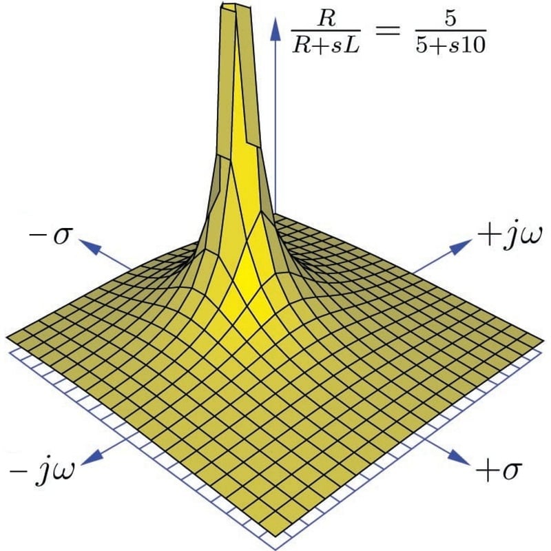
This surface plot makes the meaning of the term “pole” quite obvious: the shape of the function looks just like a rubber mat stretched up at one point by a physical pole. Here, the “pole” rises to an infinite height at a value of \(s\) where \(\sigma\) = \(-0.5\) time constants per second and \(\omega\) = 0 radians per second. The surface is seen to decrease in height at all edges of the plot, as \(\sigma\) and \(\omega\) increase in value.
The “zero” of this transfer function is not as obvious as the pole, since the function’s value does not equal zero unless and until \(s\) becomes infinite, which of course cannot be plotted on any finite domain. Suffice to say that the zero of this transfer function lies in all horizontal directions at an infinite distance away from the plot’s origin (center), explaining why the surface slopes down to zero everywhere with increasing distance from the pole.
One of the valuable insights provided by a three-dimensional pole-zero plot is the system’s response to an input signal of constant magnitude and varying frequency. This is commonly referred to as the frequency response of the system, its graphical representation called a Bode plot. We may trace the Bode plot for this system by revealing a cross-sectional slice of the three-dimensional surface along the plane where \(\sigma = 0\) (i.e. showing how the system responds to sinusoidal waves of varying frequency that don’t grow or decay over time):
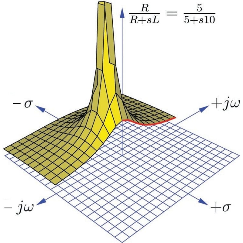
Only one-half of the pole-zero surface has been plotted here, in order to better reveal the cross-section along the \(j \omega\) axis. The bold, red curve traces the edge of the transfer function surface as it begins at zero frequency (DC) to increasingly positive values of \(j \omega\). The red trace is therefore the Bode plot for this low-pass filter, starting at a maximum value of 1 (\(V_{out} = V_{in}\) for a DC input signal) and approaching zero as frequency increases.
As insightful as three-dimensional pole-zero plots are, they are laborious to plot by hand, and even with the aid of a computer may require significant time to set up. For this reason, pole-zero plots have traditionally been drawn in a two-dimensional rather than three-dimensional format, from a “bird’s eye” view looking down at the \(s\) plane. Since this view hides any features of height, poles and zeros are instead located on the \(s\) plane by \(\times\) and \(\circ\) symbols, respectively. An example of a traditional pole-zero plot for our low-pass filter appears here:
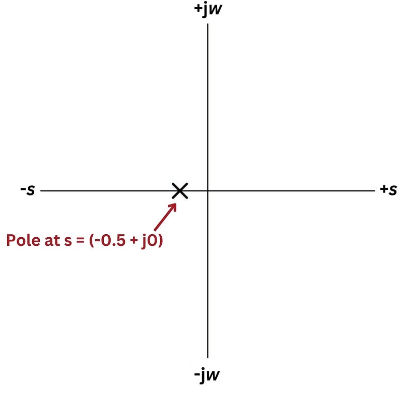
Admittedly, this type of pole-zero plot is a lot less interesting to look at than a three-dimensional surface plotted by computer, but nevertheless contains useful information about the system. The single pole lying on the real (\(\sigma\)) axis tells us the system will not self-oscillate (i.e. \(\omega = 0\) at the pole), and that it is inherently stable: when subjected to a pulse, its natural tendency is to decay to a stable value over time (i.e. \(\sigma < 0\)).
It should be noted that transfer functions and pole-zero plots apply to much more than just filter circuits. In fact, any physical system having the same “low-pass” characteristic as this filter circuit is describable by the same transfer function and the same pole-zero plots. Electric circuits just happen to be convenient applications because their individual component characteristics are so easy to represent as functions of \(s\). However, if we are able to characterize the components of a different physical system in the same terms, the same mathematical tools apply.
RC High Pass Filter Circuit
For our next exploratory example we will consider another simple filter circuit, this time comprised of a capacitor and a resistor, with the output signal taken across the resistor. As before, we may derive a transfer function by expressing \(V_{out} / V_{in}\) as a ratio of the resistor’s impedance to the total series resistor-capacitor impedance (treating this as a voltage divider circuit):
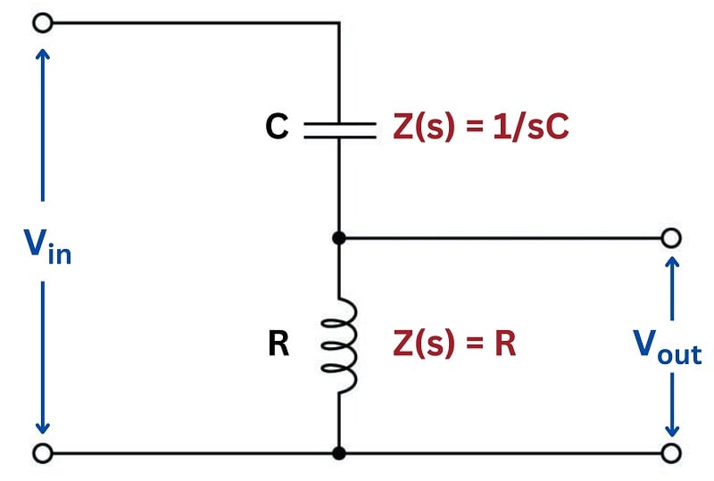
\[\hbox{Transfer function} = {V_{out}(s) \over V_{in}(s)}\]
\[{R \over {R + {1 \over sC}}}\]
High Pass Filter Transfer Function
After writing this initial transfer function based on component impedances, we will algebraically manipulate it to eliminate compound fractions. This will aid our analysis of the circuit’s DC response, zeros, and poles:
\[R \over {R + {1 \over sC}}\]
\[R \over {{sRC \over sC} + {1 \over sC}}\]
\[R \over {1 + sRC \over sC}\]
\[sRC \over 1 + sRC\]
This transfer function allows us to calculate the “gain” of the system for any given value of \(s\), which brings us to the next step of our analysis. Once again we will ask ourselves three questions about the transfer function:
- How does this system respond when \(s = 0\)?
- What value(s) of \(s\) make the transfer function approach a value of zero?
- What value(s) of \(s\) make the transfer function approach a value of infinity?
In answer to the first question, we see that the transfer function is equal to zero when \(s = 0\):
\[{0RC \over 1 + 0RC}\]
\[{0 \over 1 + 0} = {0 \over 1} = 0\]
Of course, a value of 0 for \(s\) means exposure to a steady DC signal: one that neither grows nor decays over time, nor oscillates. Therefore, this resistor-capacitor circuit will output zero voltage when exposed to a purely DC input signal. This makes conceptual sense when we examine the circuit itself: a DC input signal voltage means the capacitor will not experience any change in voltage over time, which means it will not pass any current along to the resistor. With no current through the resistor, there will be no output voltage. Thus, the capacitor “blocks” the DC input signal, preventing it from reaching the output. This behavior is exactly what we would expect from such a circuit, which any student of electronics should immediately recognize as being a simple high-pass filter: DC is a condition of zero frequency, which should be completely blocked by any filter circuit with a high-pass characteristic.
The answer to our first question is also the answer to the second question: “what value of \(s\) makes the transfer function equal to zero?” Here we see that it is only at a value of \(s = 0\) that the entire transfer function’s value will be zero. Any other values for \(s\) – even infinite – yield non-zero results. In contrast to the last circuit (the resistor-inductor low-pass filter) this circuit exhibits a singular “zero” point in its transfer function: one specific location on the pole-zero plot where the function’s value diminishes to nothing.
When we consider the third question (“What value(s) of \(s\) make the transfer function approach a value of infinity?”) we proceed the same as before: by finding value(s) of \(s\) which will make the denominator of the transfer function fraction equal to zero. If we set the denominator portion equal to zero and solve for \(s\), we will obtain the pole for the circuit:
\[1 + sRC = 0\]
\[sRC = -1\]
\[s = -{1 \over RC}\]
We know that both \(R\) and \(C\) are real numbers, not imaginary. This tells us that \(s\) will likewise be a real number at the pole. That is to say, \(s\) will be comprised of all \(\sigma\) and no \(\omega\). The fact that the value of \(\sigma\) is negative tells us the pole represents a condition of exponential decay, just the same as in the case of the resistor-inductor low-pass filter. As before, this means the circuit will produce an output voltage signal with no input voltage signal when the rate of signal decay is \(\sigma = -1 / RC\).
Recall that the rate of decay in the \(s\) variable (\(\sigma\)) is nothing more than the reciprocal of the system’s time constant (\(\tau\)). Thus, a rate of decay equal to \(1 / RC\) equates to a time constant \(\tau = RC\), which as all electronics students know is how we calculate the time constant for any simple resistor-capacitor circuit.
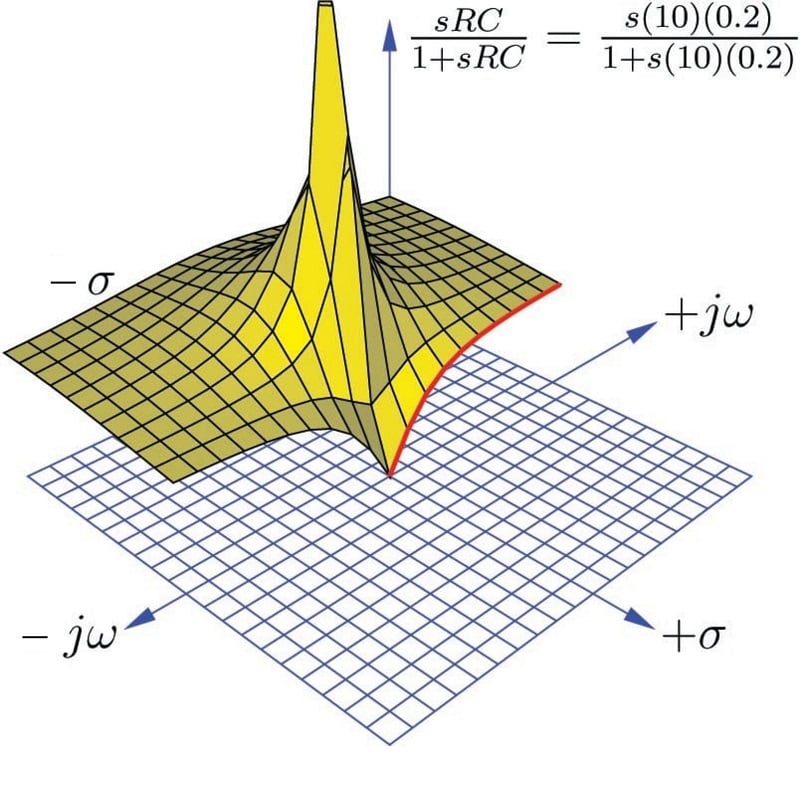
Using a computer to plot a three-dimensional representation of this transfer function, we clearly see both the pole and the zero as singularities. Here I have assumed a 10 \(\Omega\) resistor and a 0.2 F capacitor to place the pole at the same location as with the low-pass filter circuit \(s = -0.5 + j0\), for an equitable comparison:
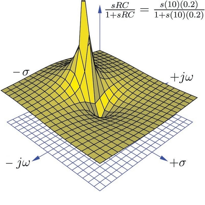
Here we see both the pole at \(s = -0.5 + j0\) and the zero at \(s = 0 + j0\) quite clearly: the pole is a singular point of infinite height while the zero is a singular point of zero height. The three-dimensional surface of the transfer function looks like a rubber sheet that has been stretched to an infinite height at the pole and stretched to ground level at the zero.
As in the last example, we may re-plot the transfer function in a way that shows a cross-sectional view at \(\sigma = 0\) in order to reveal the frequency response of this high-pass filter circuit:
Once again the bold, red curve traces the edge of the transfer function surface as it begins at zero frequency (DC) to increasingly positive values of \(j \omega\). The red trace is therefore the Bode plot for this high-pass filter, starting at a minimum value of 0 (\(V_{out} = 0\) for a DC input signal) and approaching unity (1) as frequency increases. Naturally, this is the type of response we would expect to see exhibited by a high-pass filter circuit.
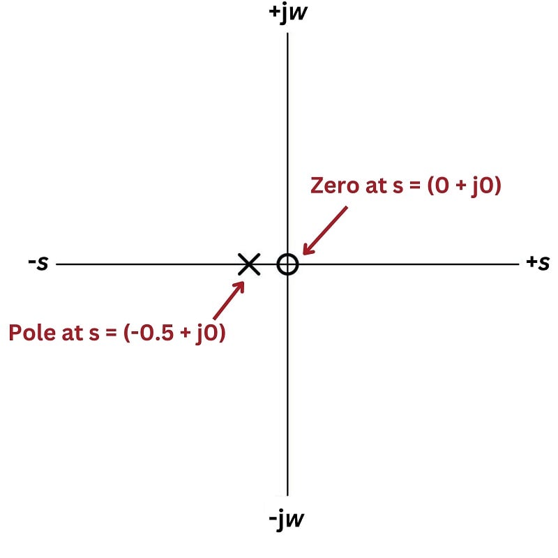
A more traditional two-dimensional pole-zero plot for this circuit locates the pole with a “\(\times\)” symbol and the zero with a “\(\circ\)” symbol:
LC Tank Circuit
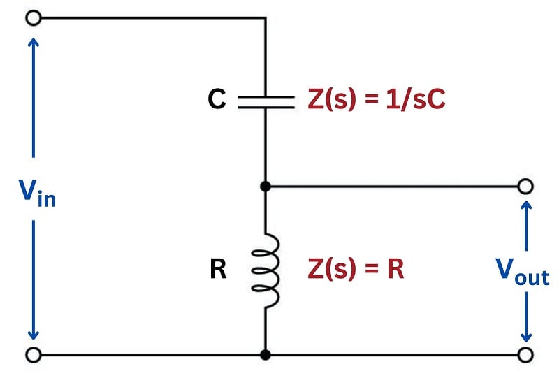
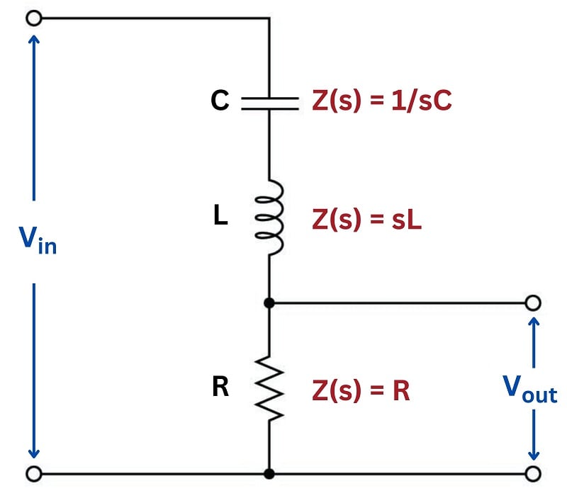
Next, we will explore the transfer function for a tank circuit, comprised of a capacitor and an inductor. We will assume the use of pure reactances here with no electrical resistance or other energy losses of any kind, just to analyze an ideal case. The output voltage in this particular circuit will be taken across the inductor:
Tank Circuit Transfer Function
Writing the transfer function for this tank circuit is (once again) a matter of expressing the ratio between the output component’s impedance versus the total circuit impedance:
\[\hbox{Transfer function} = {V_{out}(s) \over V_{in}(s)}\]
\[{sL \over {sL + {1 \over sC}}}\]
Algebraically manipulating this function to eliminate compound fractions:
\[sL \over {sL + {1 \over sC}}\]
\[sL \over {{sLsC \over sC} + {1 \over sC}}\]
\[sL \over {{s^2LC \over sC} + {1 \over sC}}\]
\[sL \over {s^2LC + 1 \over sC}\]
\[sLsC \over {s^2LC + 1}\]
\[s^2LC \over {s^2LC + 1}\]
Note how this transfer function contains \(s^2\) terms rather than \(s\) terms. This makes it a second-order function, which will yield very different results on the pole-zero plot than what we saw with either the resistor-inductor or resistor-capacitor filter circuits.
Asking ourselves the same three questions again:
- How does this system respond when \(s = 0\)?
- What value(s) of \(s\) make the transfer function approach a value of zero?
- What value(s) of \(s\) make the transfer function approach a value of infinity?
In answer to the first question, we see that the transfer function is equal to zero when \(s = 0\):
\[s^2LC \over {s^2LC + 1}\]
\[{0 \over 0 + 1} = {0 \over 1} = 0\]
As with the RC low-pass filter, its response at DC also happens to be a “zero” for the transfer function. With a DC input signal, the output signal of this circuit will be zero volts.
In order to find poles for this transfer function, we must solve for values of \(s\) that will make the denominator term of the transfer function equal to zero:
\[s^2LC + 1 = 0\]
\[s^2LC = -1\]
\[s^2 = -{1 \over LC}\]
\[s = \sqrt{-{1 \over LC}}\]
\[s = \pm j \sqrt{1 \over LC}\]
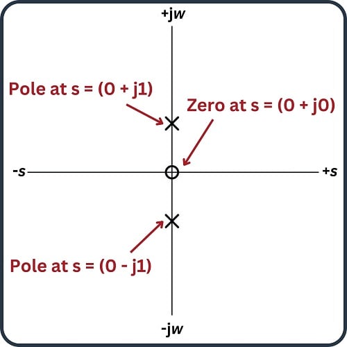
Given the fact that both \(L\) and \(C\) are real, positive numbers, and therefore solving for \(s\) requires we take the square root of a negative real number, we see that the value of \(s\) must be imaginary. We also see here that there are two poles in this transfer function: one at \(s = 0 + j \sqrt{1 \over LC}\) and another at \(s = 0 - j \sqrt{1 \over LC}\).
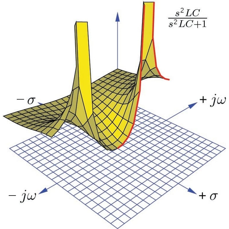
Using a computer to plot a three-dimensional representation of this transfer function, we clearly see a single zero at \(s=0\) and two poles symmetrically positioned along the \(j \omega\) axis. Here I have assumed a 0.2 F capacitor and a 5 H inductor for component values:
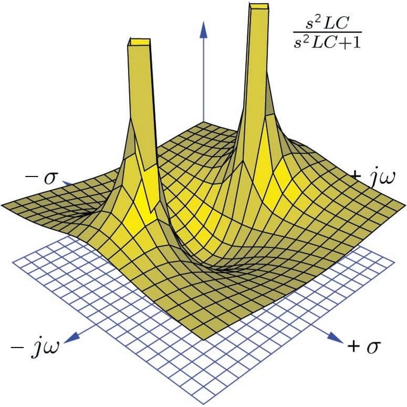
The two poles located on the \(j \omega\) axis (one at \(s = 0 + j1\) and the other at \(s = 0 - j1\)) tell us the circuit is able to generate an oscillating output signal (\(\omega\) = 1 radian per second frequency) at constant magnitude (\(\sigma = 0\)) with no input signal. This is only possible because we have assumed a perfect capacitor and a perfect inductor with no energy losses whatsoever. If we charge up either or both of these components and then immediately short-circuit the input of the circuit to ensure \(V_{in} = 0\), it will oscillate at its resonant frequency forever.
Earlier we noted that the poles in this circuit were \(s = 0 + j \sqrt{1 \over LC}\) and \(s = 0 - j \sqrt{1 \over LC}\). In other words, its resonant frequency is \(\omega = \sqrt{1 \over LC}\). Recalling that the definition for \(\omega\) is radians of phasor rotation per second, and that there are \(2 \pi\) radians in one complete revolution (cycle), we can derive the familiar resonant frequency formula for a simple LC circuit:
\[\omega = \sqrt{1 \over LC}\]
\[\hbox{. . . substituting } 2 \pi f \hbox{ for } \omega \hbox{ . . .}\]
\[2 \pi f = \sqrt{1 \over LC}\]
\[f = {1 \over 2 \pi \sqrt{LC}}\]
Taking a cross-section of this surface plot at \(\sigma = 0\) to obtain a frequency response (Bode plot) of the LC tank circuit, we see the output of this circuit begin at zero when the frequency (\(\omega\)) is zero, then the output peaks at the resonant frequency (\(\omega\) = 1 rad/sec), then the output approaches unity (1) as frequency increases past resonance:
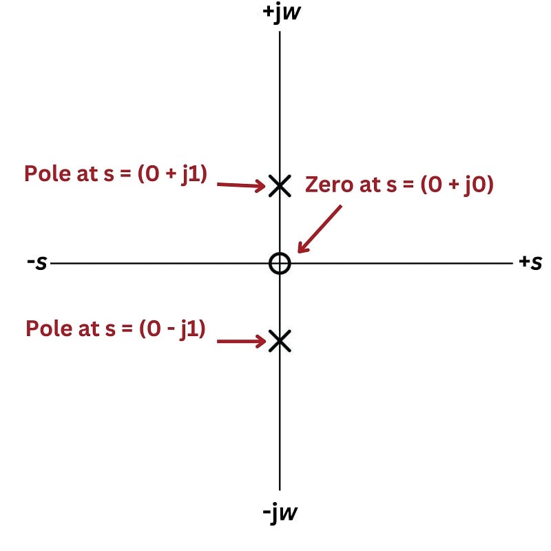
A more traditional two-dimensional pole-zero plot for this circuit locates shows the zero and the two poles using “\(\circ\)” and “\(\times\)” symbols:
RLC Band Pass Filter Circuit
For our next example circuit, we will add a resistor in series with the inductor and capacitor to explore its effects on the transfer function. Taking our output voltage across the resistor, we should expect to see band-pass filtering behavior from this circuit, with maximum voltage developing across the resistor at one frequency where the inductor’s and capacitor’s impedances cancel:
Transfer Function of an RLC Circuit
As usual, the transfer function for this circuit is the ratio between the output component’s impedance (\(R\)) and the total series impedance, functioning as a voltage divider:
\[\hbox{Transfer function} = {V_{out}(s) \over V_{in}(s)}\]
\[{R \over {R + sL + {1 \over sC}}}\]
Algebraically manipulating this function to eliminate compound fractions:
\[R \over {R + sL + {1 \over sC}}\]
\[R \over {{sRC \over sC} + {s^2LC \over sC} + {1 \over sC}}\]
\[R \over {{sRC + {s^2LC + 1} \over sC}}\]
\[sRC \over {sRC + s^2LC + 1}\]
As with the pure tank circuit analyzed previously, we can see that this LC circuit exhibits a second-order transfer function because it contains an \(s^2\) term. Running through our three questions again:
- How does this system respond when \(s = 0\)?
- What value(s) of \(s\) make the transfer function approach a value of zero?
- What value(s) of \(s\) make the transfer function approach a value of infinity?
The answers to the first two questions are one and the same: the numerator of the transfer function will be zero when \(s = 0\), this being the single zero of the function. Recalling that a condition of \(s = 0\) represents a DC input signal (no growth or decay over time, and no oscillation), this makes perfect sense: the presence of the DC-blocking series capacitor in this circuit ensures the output voltage under steady-state conditions must be zero.
In answering the third question to identify any poles for this circuit, we encounter a more complicated mathematical problem than seen with previous example circuits. The denominator of the transfer function’s fraction is a second-degree polynomial in the variable \(s\). As you may recall from your study of algebra, any solution resulting in a polynomial having an over-all value of zero is called a root of that polynomial expression. Since this particular expression is found in the denominator of the transfer function where we know zero values mark poles of the system, and solutions for \(s\) resulting are roots of the polynomial, then roots of the expression \(sRC + s^2LC + 1\) must mark the locations of the poles on the \(s\) plane.
A very useful algebraic tool for finding roots of a second-degree polynomial expression is the quadratic formula:
\[x = {{-b \pm \sqrt{b^2 - 4ac}} \over 2a}\]
Where:
\(ax^2 + bx + c\) is a polynomial expression
\(x\) is the independent variable of that polynomial expression
\(a\) is the coefficient of the second-degree (\(x^2\)) term
\(b\) is the coefficient of the first-degree (\(x\)) term
\(c\) is the coefficient of the zero-degree (constant) term
Reviewing the denominator of our transfer function again, we see that \(s\) is the independent variable, and so \(LC\) must be the “\(a\)” coefficient, \(RC\) must be the “\(b\)” coefficient, and 1 must be the “\(c\)” coefficient. Substituting these variables into the quadratic formula will give us a formula for computing the poles of this resistor-inductor-capacitor circuit:
\[s = {{-RC \pm \sqrt{(RC)^2 - 4LC}} \over 2LC}\]
Perhaps the most interesting part of this formula is what lies beneath the radicand (square-root) symbol: \((RC)^2 - 4LC\). This portion of the quadratic formula is called the discriminant, and its value determines both the number of roots as well as their real or imaginary character. If the discriminant is equal to zero, there will be a single real root for our polynomial and therefore only one pole for our circuit. If the discriminant is greater than zero (i.e. a positive value), then there will be two real roots and therefore two poles lying on the \(\sigma\) axis (i.e. no imaginary \(j \omega\) parts). If the discriminant is less than zero (i.e. a negative value), then there will be two complex roots for our polynomial and therefore two complex poles having both real and imaginary parts.
Let us consider for a moment what the sign of the discriminant means in practical terms. A pole that is purely real means a value for \(s\) that is all \(\sigma\) and no \(\omega\): representing a condition of growth or decay but with no oscillation. This is similar to what we saw with the LR or RC low/high pass filter circuits, where the circuit in a state of discharge could generate an output signal even with its input terminals shorted to ensure no input signal.
If we have a positive value for the discriminant which yields two real poles, it means two different possible values for \(\sigma\) (rate of growth/decay) that could occur with no signal input to the circuit. This behavior is only possible with two energy-storing components in the circuit: a kind of double time-constant where different portions of the circuit discharge at different rates. The lack of any imaginary part within \(s\) means the circuit still will not self-oscillate.
If we have a negative value for the discriminant which yields two complex poles, it means two different values for \(s\) both having real and imaginary parts. Since the real part (\(\sigma\)) represents growth/decay while the imaginary part (\(\omega\)) represents oscillation, complex poles tell us the circuit will be able to self-oscillate but not at a constant magnitude as with an ideal (lossless) tank circuit. In fact, intuition should tell us these complex poles must have negative real values representing decaying oscillations, because it would violate the Law of Energy Conservation for our circuit to self-oscillate with increasing magnitude.
Looking at the discriminant \((RC)^2 - 4LC\) we see that it is possible to push the circuit into any one of these three modes of operation merely by adjusting the value of \(R\) and leaving both \(L\) and \(C\) unchanged. If we wish to calculate the critical value of \(R\) necessary to produce a single real pole for any given values of \(L\) and \(C\), we may set the discriminant equal to zero and algebraically solve for \(R\) as follows:
\[(RC)^2 - 4LC = 0\]
\[(RC)^2 = 4LC\]
\[RC = \sqrt{4LC}\]
\[RC = 2 \sqrt{L} \sqrt{C}\]
\[R = {2 \sqrt{L} \sqrt{C} \over C}\]
\[R = {{2 \sqrt{L} \sqrt{C}} \over {\sqrt{C} \sqrt{C}}}\]
\[R = {2 \sqrt{L} \over \sqrt{C}} = 2 \sqrt{L \over C}\]
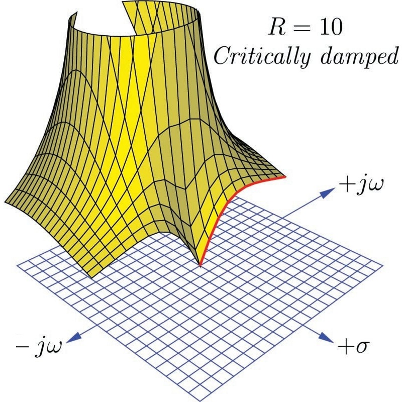
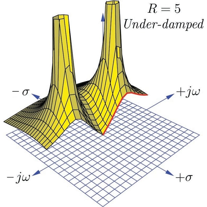
This critical value of \(R\) resulting in one real pole is the minimum amount of resistance necessary to prevent self-oscillation. If the circuit is operating at this point, it is said to be critically damped. Larger values of \(R\) will result in multiple real poles, where the circuit is said to be over-damped. Smaller values of \(R\) will permit some self-oscillation to occur, and the circuit is said to be under-damped.
Sometimes electrical engineers intentionally install resistors into circuits containing both inductance and capacitance for the express purpose of damping oscillations. In such cases, the resistor is called an anti-resonance resistor, because its purpose is to combat resonant oscillations that would otherwise occur as the inductive and capacitive elements of the circuit exchange energy back and forth with each other. If the engineer’s intent is to install just enough resistance into the circuit to prevent oscillations without creating unnecessary time delays, then the best value of the resistor will be that which causes critical damping.
Recall that the subject of transfer functions, poles, and zeros applies to any linear system, not just AC circuits. Mechanical systems, feedback control loops, and many other physical systems may be characterized in the same way using the same mathematical tools. This particular subject of damping is extremely important in applications where oscillations are detrimental. Consider the design of an automobile’s suspension system, where the complementary energy-storing phenomena of spring tension and vehicle mass give rise to oscillations following impact with a disturbance in the road surface. It is the job of the shock absorber to act as the “resistor” in this system and dissipate energy in order to minimize oscillations following a bump in the road. An under-sized shock absorber won’t do a good enough job dissipating the energy of the disturbance, and so the vehicle’s suspension will exhibit complex poles (i.e. there will be some lingering oscillations following a bump). An over-sized shock absorber will be too “stiff” and allow too much of the bump’s energy to pass through to the vehicle frame and passengers. A perfectly-sized shock absorber, however, will “critically damp” the system to completely prevent oscillation while presenting the smoothest ride possible.
Likewise, oscillations following a disturbance are undesirable in a feedback control system where the goal is to maintain a process variable as close to setpoint as possible. An under-damped feedback loop will tend to oscillate excessively following a disturbance. An over-damped feedback loop won’t oscillate, but it will take an excessive amount of time to converge back on setpoint which is also undesirable because this means more time spent off setpoint. A critically-damped feedback loop is the best-case compromise, where oscillations are eliminated and convergence time is held to a minimum.
In order to fully illustrate the characteristics of this circuit’s transfer function, we will do so for three different resistor values: one where \(R\) yields critical damping (one real pole), one where \(R\) makes the circuit over-damped (two real poles), and one where \(R\) makes the circuit under-damped (two complex poles). We will use three-dimensional plotting to show the transfer function response in each case. To be consistent with our former tank circuit example, we will assume the same capacitor value of 0.2 Farads and the same inductor value of 5 Henrys. The resistor value will be modified in each case to create a different damping condition.
First, the critically-damped example, with a resistor value of 10 ohms:
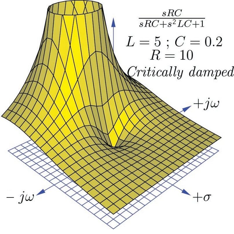
As expected, a single zero appears at \(s = 0\), and a single pole at \(s = -1 + j0\). Thus, this circuit has a decay rate of -1 time constants per second (\(\tau\) = 1 second) as seen when we use the quadratic formula to solve for \(s\):
\[s = {{-RC \pm \sqrt{(RC)^2 - 4LC}} \over 2LC}\]
\[s = {{-(10)(0.2) \pm \sqrt{[(10)(0.2)]^2 - (4)(5)(0.2)}} \over (2)(5)(0.2)}\]
\[s = {{-2 \pm \sqrt{0}} \over 2} = (-1 + j0) \hbox{ sec}^{-1}\]
Interestingly, only \(L\) and \(R\) determine the decay rate (\(\sigma\), the real part of \(s\)) in the critically damped condition. This is clear to see if we set the discriminant to zero in the quadratic formula and look for variables to cancel:
\[s = {{-RC \pm \sqrt{0}} \over 2LC} = -{R \over 2L}\]
Next, we will plot the same transfer function with a larger resistor value (15 ohms) to ensure over-damping:
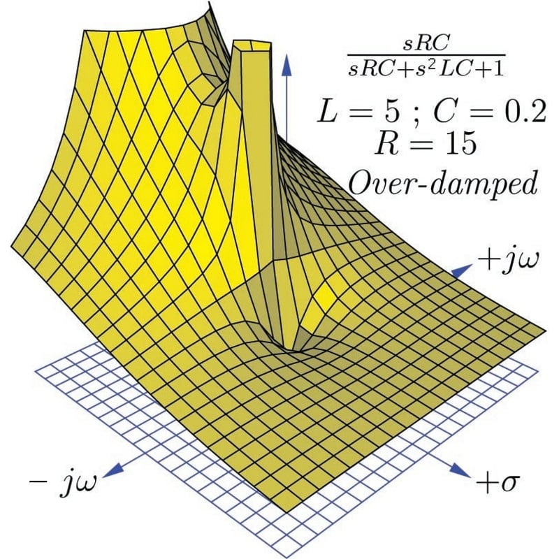
We clearly see two poles centered along the \(\sigma\) axis in this plot, representing the two real roots of the transfer function’s denominator. Again, we will use the quadratic formula to solve for these two values of \(s\):
\[s = {{-RC \pm \sqrt{(RC)^2 - 4LC}} \over 2LC}\]
\[s = {{-(15)(0.2) \pm \sqrt{[(15)(0.2)]^2 - (4)(5)(0.2)}} \over (2)(5)(0.2)}\]
\[s = {{-3 \pm \sqrt{(3)^2 - 4}} \over 2}\]
\[s = {{-3 + \sqrt{5}} \over 2} = (-0.382 + j0) \hbox{ sec}^{-1}\]
\[s = {{-3 - \sqrt{5}} \over 2} = (-2.618 + j0) \hbox{ sec}^{-1}\]
These real poles represent two different decay rates (time constants) for the over-damped circuit: a fast decay rate of \(\sigma = -2.618\) sec\(^{-1}\) and a slow decay rate of \(\sigma = -0.382\) sec\(^{-1}\), the slower of these two decay rates dominating the circuit’s transient response over long periods of time.
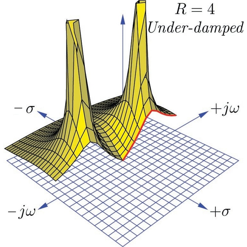
Next, we will plot the same transfer function with a smaller resistor value (5 ohms) to ensure under-damping:
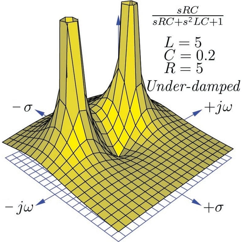
We clearly see two poles once again, but neither of them are located on an axis. These represent two complex values for \(s\) describing the circuit’s behavior with zero input. The imaginary (\(j \omega\)) part of \(s\) tells us the circuit has the ability to self-oscillate. The negative, real (\(\sigma\)) part of \(s\) tells us these oscillations decrease in magnitude over time. Using the quadratic formula to solve for these two poles:
\[s = {{-RC \pm \sqrt{(RC)^2 - 4LC}} \over 2LC}\]
\[s = {{-(5)(0.2) \pm \sqrt{[(5)(0.2)]^2 - (4)(5)(0.2)}} \over (2)(5)(0.2)}\]
\[s = {{-1 \pm \sqrt{(1)^2 - 4}} \over 2}\]
\[s = {{-1 + \sqrt{-3}} \over 2} = (-0.5 + j0.866) \hbox{ sec}^{-1}\]
\[s = {{-1 - \sqrt{-3}} \over 2} = (-0.5 - j0.866) \hbox{ sec}^{-1}\]
The calculated \(\omega\) value of 0.866 radians per second is slower than the 1 radian per second resonant frequency calculated for the pure tank circuit having the same \(L\) and \(C\) values, revealing that the damping resistor skews the “center” frequency of this RLC band-pass filter. The calculated \(\sigma\) value of \(-0.5\) time constants per second (equivalent to a time constant of \(\tau\) = 2 seconds) describes the rate at which the sinusoidal oscillations decay in magnitude. Here as well we see the under-damped decay rate (\(\sigma = -0.5\) sec\(^{-1}\)) is slower than the critically damped decay rate (\(\sigma = -1\) sec\(^{-1}\)).
If we compare two-dimensional pole-zero plots for each of the three resistor values in this RLC circuit, we may contrast the over-damped, critically-damped, and under-damped responses:
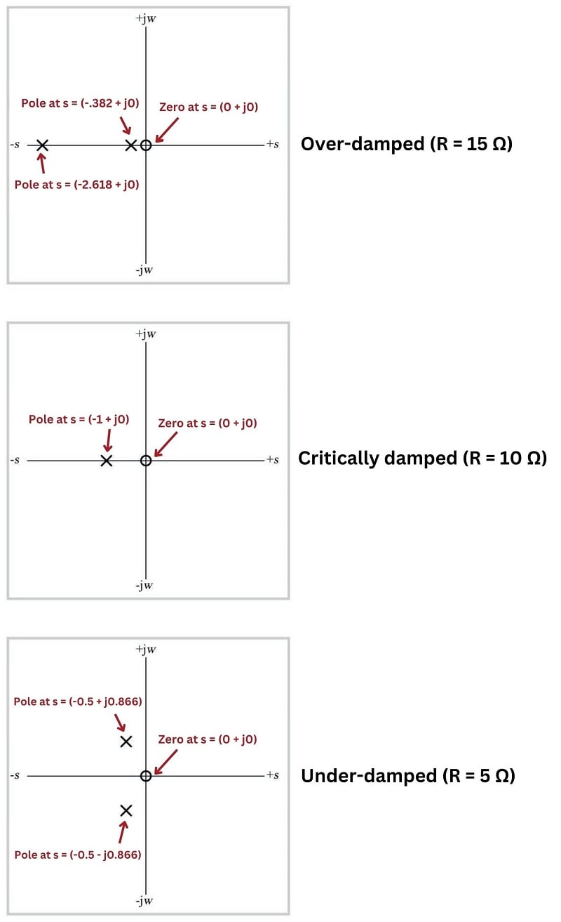
(Click to see expanded view)
If we take cross-sectional plots of the transfer function at \(\sigma = 0\) to show the frequency response of this RLC band-pass filter, we see the response become “sharper” (more selective) as the resistor’s value decreases and the poles move closer to the \(j \omega\) axis. Electronic technicians relate this to the quality factor or \(Q\) of the band-pass filter circuit, the circuit exhibiting a higher “quality” of band-pass selection as the ratio of reactance to resistance increases:
(Click on any image below to see an expanded view)
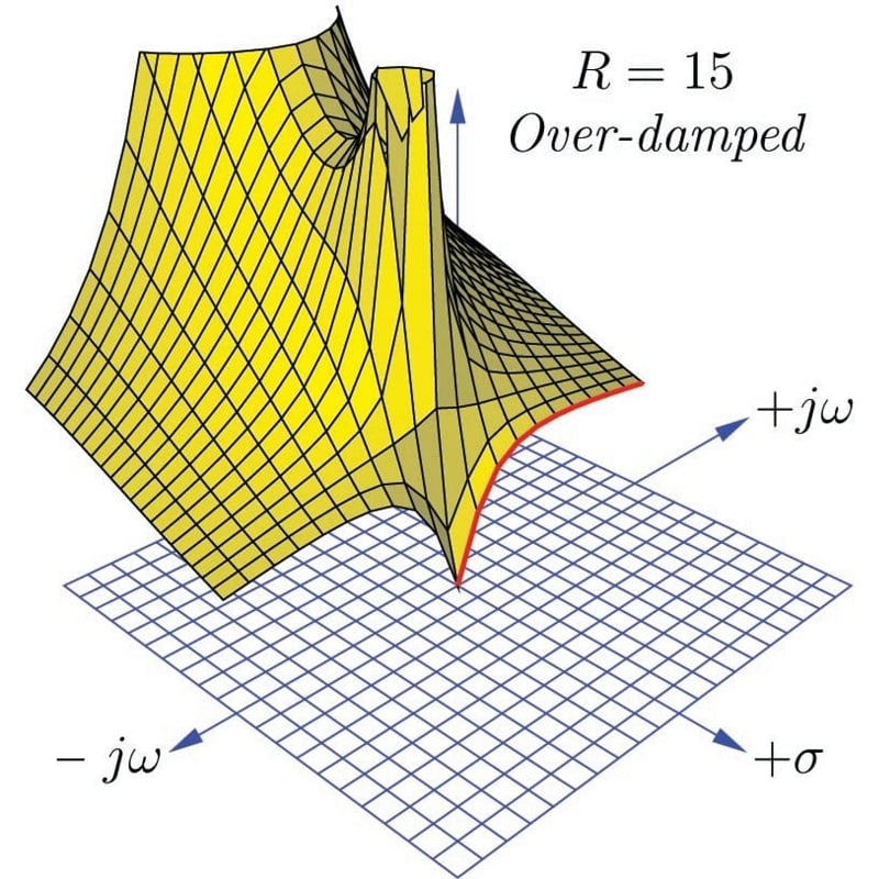
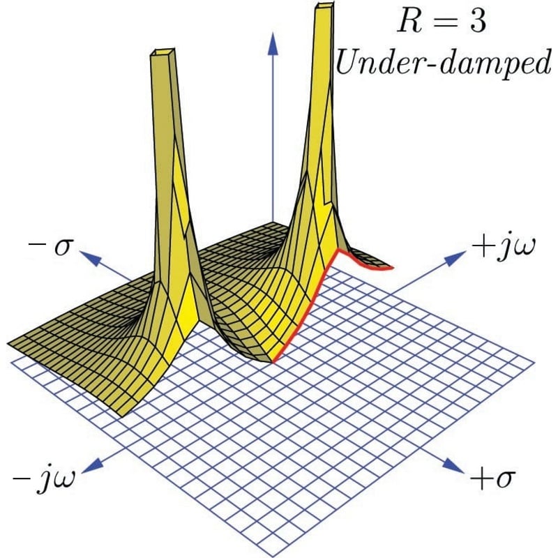
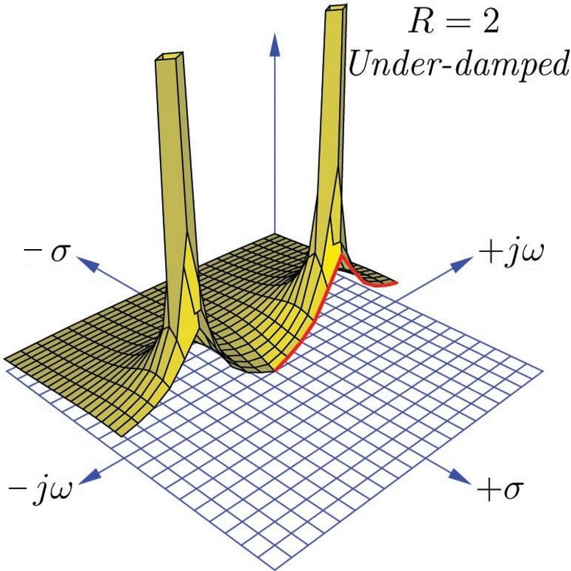
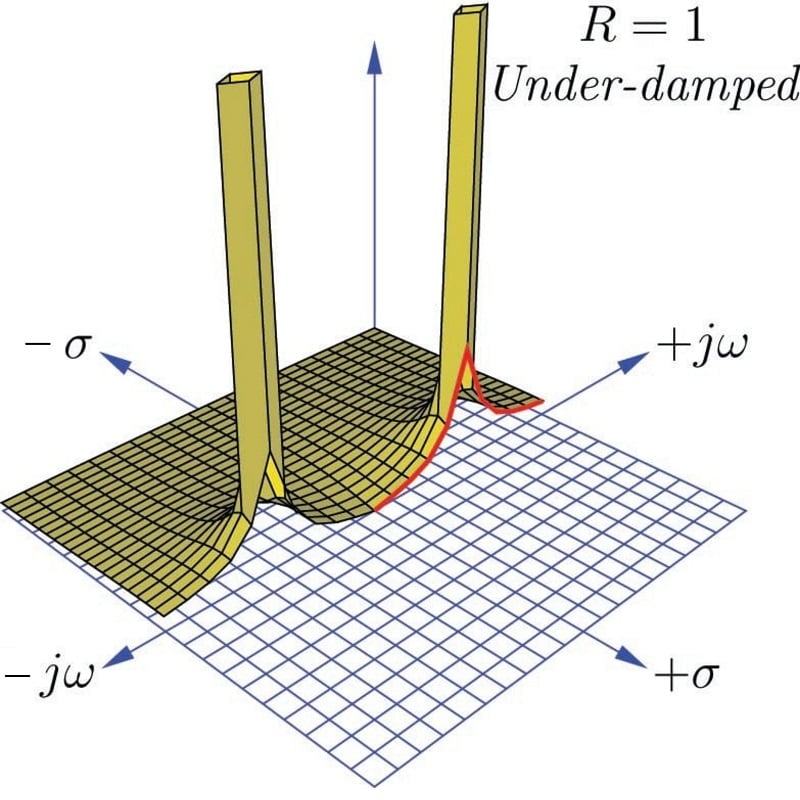
Although each and every pole in a pole-zero plot is has the same (infinite) height, poles grow narrower when moved farther away from each other, and wider when closely spaced. As the resistance in this circuit decreases and the poles move farther away from each other and closer to the \(j \omega\) axis, their widths narrow and the frequency response curve’s peak becomes narrower and steeper.
Summary of Transfer Function Analysis
Here is a summary of some of the major concepts important to transfer function analysis:
- The \(s\) variable is an expression of growing/decaying sinusoidal waves, comprised of a real part and an imaginary part (\(s = \sigma + j \omega\)). The real part of \(s\) (\(\sigma\)) is the growth/decay rate, telling us how rapidly the signal grows or decays over time, with positive values of \(\sigma\) representing growth and negative values of \(\sigma\) representing decay. This growth/decay rate is the reciprocal of time constant (\(\sigma = 1 / \tau\)), and is measured in reciprocal units of time (time constants per second, or sec\(^{-1}\)). The imaginary part of \(s\) (\(j \omega\)) represents the frequency of the sinusoidal quantity, measured in radians per second (sec\(^{-1}\)).
- An important assumption we make when analyzing any system’s transfer function(s) is that the system is linear (i.e. its output and input magnitudes will be proportional to each other for all conditions) and time-invariant (i.e. the essential characteristics of the system do not change with the passage of time). If we wish to analyze a non-linear system using these tools, we must limit ourselves to ranges of operation where the system’s response is approximately linear, and then accept small errors between the results of our analysis and the system’s real-life response.
- For any linear time-invariant system (an “LTI” system), \(s\) is descriptive throughout the system. In other words, for a certain value of \(s\) describing the input to this system, that same value of \(s\) will also describe the output of that system.
- A transfer function is an expression of a system’s gain, measured as a ratio of output over input. In engineering, transfer functions are typically mathematical functions of \(s\) (i.e. \(s\) is the independent variable in the formula). When expressed in this way, the transfer function for a system tells us how much gain the system will have for any given value of \(s\).
- Transfer functions are useful for analyzing the behavior of electric circuits, but they are not limited to this application. Any linear system, whether it be electrical, mechanical, chemical, or otherwise, may be characterized by transfer functions and analyzed using the same mathematical techniques. Thus, transfer functions and the \(s\) variable are general tools, not limited to electric circuit analysis.
- A zero is any value of \(s\) that results in the transfer function having a value of zero (i.e. zero gain, or no output for any magnitude of input). This tells us where the system will be least responsive. On a three-dimensional pole-zero plot, each zero appears as a low point where the surface touches the \(s\) plane. On a traditional two-dimensional pole-zero plot, each zero is marked with a circle symbol (\(\circ\)). We may solve for the zero(s) of a system by solving for value(s) of \(s\) that will make the numerator of the transfer function equal to zero, since the numerator of the transfer function represents the output term of the system.
- A pole is any value of \(s\) that results in the transfer function having an infinite value (i.e. maximum gain, yielding an output without any input). This tells us what the system is capable of doing when it is not being “driven” by any input stimulus. Poles are typically associated with energy-storing elements in a passive system, because the only way an unpowered system could possibly generate an output with zero input is if there are energy-storing elements within that system discharging themselves to the output. On a three-dimensional pole-zero plot, each pole appears as a vertical spike on the surface reaching to infinity. On a traditional two-dimensional pole-zero plot, each pole is marked with a (\(\times\)) symbol. We may solve for the pole(s) of a system by solving for value(s) of \(s\) that will make the denominator of the transfer function equal to zero, since the denominator of the transfer function represents the input term of the system.
- Second-order systems are capable of self-oscillation. This is revealed by poles having imaginary values. These oscillations may be completely undamped (i.e. \(s\) is entirely imaginary, with \(\sigma = 0\)), in which case the system is able to oscillate forever on its own. If energy-dissipating elements are present in a second-order system, the oscillations will be damped (i.e. decay in magnitude over time).
- An under-damped system exhibits complex poles, with \(s\) having both imaginary (\(j \omega\)) frequency values and real (\(\sigma\)) decay values. This means the system can self-oscillate, but only with decreasing magnitude over time.
- A critically damped system is one having just enough dissipative behavior to completely prevent self-oscillation, exhibiting a single pole having only a real (\(\sigma\)) value and no imaginary (\(j \omega\)) value.
- An over-damped system is one having excessive dissipation, exhibiting multiple real poles. Each of these real poles represents a different decay rate (\(\sigma\)) or time constant (\(\tau = 1 / \sigma\)) in the system. When these decay rates differ in value substantially from one another, the slowest one will dominate the behavior of the system over long periods of time.

thank a lot! so clear so easy you did a wonderful works!
hard topics with easiest way