 Facebook
 Google
 GitHub
 Linkedin
Open-ended, Shorted, and Properly Terminated Transmission Lines
Cable impedance is not a matter of length, material, or diameter as for most resistance measurements
Cable impedance is a critical property that provides a state of loading for short durations in transmission lines that carry waveforms, including popular 50-ohm and 75-ohm impedance coax cables.
Many years ago, when I was first learning about electricity, I happened to discover a length of coaxial television cable with the rating “50 ohm” printed on the jacket.
What is 50 Ohm Cable?
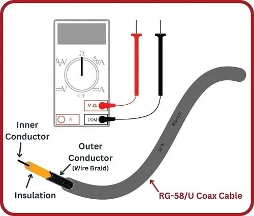
Having my own ohmmeter, and wanting to know what the “50 ohm” label referred to, I tried measuring the resistance of this cable to see where it would exhibit 50 ohms of resistance. First I tried measuring between the two open-ended wires (the center conductor and the braided shield conductor), where my meter registered infinite resistance (no continuity). This is what I expected a normal cable would read when connected to nothing else. Next, I tried connecting my meter from one end of the cable to the other: between both ends of the center conductor, and my meter registered 0 ohms. Between both ends of the shield conductor, my meter also read 0 ohms. In fact, this is all I was ever able to measure with my ohmmeter: either 0 ohms or infinite ohms (open), no matter what I tried. I was confounded – how could this piece of cable possibly be called a “50 ohm” cable if I could not measure 50 ohms anywhere on it?
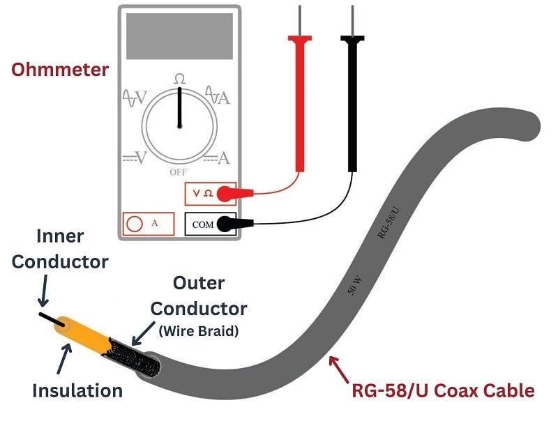
It was not until years later that I came across a reference in an old book to something called surge impedance, describing how lengths of cable responded to short-duration electrical pulses, that I finally understood the “50 ohm” rating of that coaxial cable. What I failed to discover with my ohmmeter – in fact, what I never could have even seen with a plain ohmmeter – is that the cable did indeed act like a 50 ohm resistor, but only for extremely short periods of time. This is an aspect of electrical theory I was completely unprepared to comprehend at that time, knowing only how DC circuits functioned. This is the subject we are about to explore now.
Characteristic Impedance of a Cable
In basic DC electrical theory, students learn that open circuits always drop the full applied voltage and cannot have electric currents anywhere in them. Students likewise learn that short circuits drop negligible voltage while conducting full electrical current. They also learn that the effects of electricity occur instantaneously throughout the circuit: for example, if a functioning circuit suffers an “open” fault, current through that branch of the circuit halts immediately and everywhere. These basic rules of electricity are extremely useful for DC circuit analysis, indeed even essential for troubleshooting DC circuits, but they are not 100% correct. Like many of the scientific principles one initially learns, they are only approximations of reality.
The effects of electricity do not propagate instantaneously throughout a circuit, but rather spread at the speed of light (approximately 300,000,000 meters per second). Normally we never see any consequences of this finite speed because everything happens so fast, just as I never saw my ohmmeter register 50 ohms when I tried to test that coaxial cable many years ago. However, when we test a circuit on a time scale of nano-seconds (billionths of a second!), we find some very interesting phenomena during the time electricity propagates along the length of a circuit: open circuits can indeed (temporarily) exhibit current, and short circuits can indeed (temporarily) exhibit voltage drops.
When a pulse signal is applied to the beginning of a two-conductor cable, the reactive elements of that cable (i.e. capacitance between the conductors, inductance along the cable length) begin to store energy. This translates to a current drawn by the cable from the source of the pulse, as though the cable were acting as a (momentarily) resistive load. If the cable under test were infinitely long, this charging effect would never end, and the cable would indeed behave exactly like a resistor from the perspective of the signal source. However, real cables (having finite length) do stop “charging” after some time following the application of a voltage signal at one end, the length of that time being a function of the cable’s physical length and the speed of light.
In honor of the cable’s capacity to behave as a temporary load to any impressed signal, we typically refer to it as something more than just a cable. From the perspective of an electrical pulse, measured on a time scale of nanoseconds, we refer to any cable as a transmission line. All electrical cables act as transmission lines, but the effects just mentioned are so brief in duration that we only notice them when the cable is exceptionally long and/or the pulse durations are exceptionally short (i.e. high-frequency signals).
Surge Impedance Loading
During the time when a transmission line is absorbing energy from a power source – whether this is indefinitely for a transmission line of infinite length, or momentarily for a transmission line of finite length – the current it draws will be in direct proportion to the voltage applied by the source. In other words, a transmission line behaves like a resistor, at least for a moment. The amount of “resistance” presented by a transmission line is called its characteristic impedance, or surge impedance, symbolized in equations as \(Z_0\). Only after the pulse signal has had time to travel down the length of the transmission line and reflect back to the source does the cable stop acting as a load and begin acting as a plain pair of wires.
A transmission line’s characteristic impedance is a function of its conductor geometry (wire diameter, spacing) and the permittivity of the dielectric separating those conductors. If the line’s design is altered to increase its bulk capacitance and/or decrease its bulk inductance (e.g. decreasing the distance between conductors), the characteristic impedance will decrease. Conversely, if the transmission line is altered such that its bulk capacitance decreases and/or its bulk inductance increases, the characteristic impedance will increase. It should be noted that the length of the transmission line has absolutely no bearing on characteristic impedance. A 10-meter length of RG-58/U coaxial cable will have the exact same characteristic impedance as a 10,000-kilometer length of RG-58/U coaxial cable (50 ohms, in both cases). The only difference is the length of time the cable will behave like a resistor to an applied voltage.
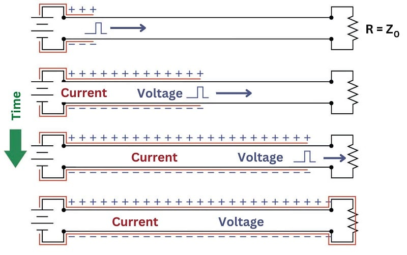
Open-ended Transmission Line Voltage
The following sequence illustrates the propagation of a voltage pulse forward and back (reflected) on an open-ended transmission line beginning from the time the DC voltage source is first connected to the left-hand end:

The end result is a transmission line exhibiting the full source voltage, but no current. This is exactly what we would expect in an open circuit. However, during the time it took for the pulse to travel down the line’s length and back, it drew current from the source equal to the source voltage divided by the cable’s characteristic impedance (\(I_{surge} = {V_{source} \over Z_0}\)). For a brief amount of time, the two-conductor transmission line acted as a load to the voltage source rather than an open circuit. Only after the pulse traveled down the full length of the line and back did the line finally act as a plain open circuit.
An experiment performed with a square-wave signal generator and oscilloscope connected to one end of a long wire pair cable (open on the far end) shows the effect of the reflected signal:

The waveform steps up for a brief time, then steps up further to full source voltage. The first step represents the voltage at the source during the time the pulse traveled along the cable’s length, when the cable’s characteristic impedance acted as a load to the signal generator (making its output voltage “sag” to a value less than its full potential). The next step represents the reflected pulse’s return to the signal generator, when the cable’s capacitance is fully charged and is no longer drawing current from the signal generator (making its output voltage “rise”). A two-step “fall” appears at the trailing edge of the pulse, when the signal generator reverses polarity and sends an opposing pulse down the cable.
The duration of the first and last “steps” on the waveform represents the time taken by the signal to propagate down the length of the cable and return to the source. This oscilloscope’s timebase was set to 0.5 microseconds per division for this experiment, indicating a pulse round-trip travel time of approximately 0.2 microseconds. A cable of this type has a velocity factor of approximately 0.7, which means electrical impulses travel at only 70% the speed of light through the cable, and so the round-trip distance calculates to be approximately 42 meters which makes the cable 21 meters in length:
\[\hbox{Distance} = \hbox{Velocity} \times \hbox{Time} = (70\%) (3 \times 10^8 \hbox{ m/s}) (0.2 \> \mu \hbox{s}) = 42 \hbox{ m}\]
\[\hbox{Cable length} = {1 \over 2} (\hbox{Distance traveled by pulse}) = (0.5)(42 \hbox{ m}) = 21 \hbox{ m}\]
Shorted Transmission Lines
The following sequence illustrates the propagation of a voltage pulse forward and back (reflected) on a shorted-end transmission line beginning from the time the DC voltage source is first connected to the left-hand end:

The end result is a transmission line exhibiting the full current of the source (\(I_{max} = {V_{source} \over R_{wire}}\)), but no voltage. This is exactly what we would expect in a short circuit. However, during the time it took for the pulse to travel down the line’s length and back, it drew current from the source equal to the source voltage divided by the cable’s characteristic impedance (\(I_{surge} = {V_{source} \over Z_0}\)). For a brief amount of time, the two-conductor transmission line acted as a moderate load to the voltage source rather than a direct short. Only after the pulse traveled down the full length of the line and back did the line finally act as a plain short-circuit.
An experiment performed with the same signal generator and oscilloscope connected to one end of the same long wire pair cable (shorted on the far end) shows the effect of the reflected signal:

Here, the waveform steps up for a brief time, then steps down toward zero. As before, the first step represents the voltage at the source during the time the pulse traveled along the cable’s length, when the cable’s characteristic impedance acted as a load to the signal generator (making its output voltage “sag” to a value less than its full potential). The step down represents the (inverted) reflected pulse’s return to the signal generator, nearly canceling the incident voltage and causing the signal to fall toward zero. A similar pattern appears at the trailing edge of the pulse, when the signal generator reverses polarity and sends an opposing pulse down the cable.
Note the duration of the pulse on this waveform, compared to the first and last “steps” on the open-circuited waveform. This pulse width represents the time taken by the signal to propagate down the length of the cable and return to the source. This oscilloscope’s timebase remained at 0.5 microseconds per division for this experiment as well, indicating the same pulse round-trip travel time of approximately 0.2 microseconds. This stands to reason, as the cable length was not altered between tests; only the type of termination (short versus open).
Properly Terminated Transmission Lines
Proper “termination” of a transmission line consists of connecting a resistance to the end(s) of the line so that the pulse “sees” the exact same amount of impedance at the end as it did while propagating along the line’s length. The purpose of the termination resistor is to completely dissipate the pulse’s energy in order that none of it will be reflected back to the source.
The following sequence illustrates the propagation of a voltage pulse on a transmission line with proper “termination” (i.e. a resistor matching the line’s surge impedance, connected to the far end) beginning from the time the DC voltage source is first connected to the left-hand end:
From the perspective of the pulse source, this properly terminated transmission line “looks” the same as an unterminated line of infinite length. There is no reflected pulse, and the DC voltage source “sees” an unchanging load resistance the entire time.
An experiment performed with a termination resistor in place shows the near-elimination of reflected pulses:

The pulse looks much more like the square wave it should be, now that the cable has been properly terminated. With the termination resistor in place, a transmission line always presents the same impedance to the source, no matter what the signal level or the time of signal application. Another way to think of this is from the perspective of cable length. With the proper size of termination resistor in place, the cable appears infinitely long from the perspective of the power source because it never reflects any signals back to the source and it always consumes power from the source.
Termination Resistors for RS-485 Lines
Data communication cables for digital instruments behave as transmission lines, and must be terminated at both ends to prevent signal reflections. Reflected signals (or “echoes”) may cause errors in received data in a communications network, which is why proper termination can be so important. For point-to-point networks (networks formed by exactly two electronic devices, one at either end of a single cable), the proper termination resistance is often designed into the transmission and receiving circuitry, and so no external resistors need be connected. For “multi-drop” networks where multiple electronic devices tap into the same electrical cable, excessive signal loading would occur if each and every device had its own built-in termination resistance, and so the devices are built with no internal termination, and the installer must place two termination resistors in the network (one at each far end of the cable).
Transmission Line Discontinuity
A transmission line’s characteristic impedance will be constant throughout its length so long as its conductor geometry and dielectric properties are consistent throughout its length. Abrupt changes in either of these parameters, however, will create a discontinuity in the cable capable of producing signal reflections. This is why transmission lines must never be sharply bent, crimped, pinched, twisted, or otherwise deformed.
The probe for a guided-wave radar (GWR) liquid level transmitter is another example of a transmission line, one where the vapor/liquid interface creates a discontinuity: there will be an abrupt change in characteristic impedance between the transmission line in vapor space versus the transmission line submerged in a liquid due to the differing dielectric permittivities of the two substances. This sudden change in characteristic impedance sends a reflected signal back to the transmitter. The time delay measured between the signal’s transmission and the signal’s reception by the transmitter represents the vapor space distance, or ullage.
Velocity factor
The speed at which an electrical signal propagates down a transmission line is never as fast as the speed of light in a vacuum, owing to the permittivity of the line’s electrical insulation being greater than that of a vacuum. A value called the velocity factor expresses the propagation velocity as a ratio to light, and its value is always less than one:
\[\hbox{Velocity factor} = {v \over c}\]
Where,
\(v\) = Propagation velocity of signal traveling along the transmission line
\(c\) = Speed of light in a vacuum (\(\approx\) 3.0 \(\times\) \(10^8\) meters per second)
Velocity factor is a function of dielectric constant, but not conductor geometry. A greater permittivity value results in a slower velocity (lesser velocity factor).
Transmission Line Losses
Ideally, a transmission line is a perfectly loss-less conduit for electrical energy. That is, every watt of signal power entering the transmission line is available at the end where the load is connected. In reality, though, this is never the case. Conductor resistance, as well as losses within the dielectric (insulating) materials of the cable, rob the signal of energy.
Power Loss in Transmission Lines
For transmission lines, power loss is typically expressed in units of decibels per 100 feet or per 100 meters. A “decibel,” as you may recall, is ten times the logarithm of a power ratio:
\[\hbox{Gain or Loss in dB} = 10 \log \left({P \over P_{ref}}\right)\]
Thus, if a transmission line receives 25 milliwatts of signal power at one end, but only conveys 18 milliwatts to the far end, it has suffered a 1.427 dB loss (\(10 \log {0.018 \over 0.025}\) = \(-1.427\) dB) from end to end. Power loss in cables is strongly dependent on frequency: the greater the signal frequency, the more severe the power loss per unit cable length.
REVIEW:
-
Standard cables exhibit infinite ohms (no current) between conductors in a disconnected cable.
-
Likewise, standard ideal cables exhibit 0 ohms of resistance through each conductor from end-to-end.
-
Multi-conductor cables with capacitance between conductors allow current to flow momentarily when the applied voltage changes, such as with an AC waveform.
-
Transmission lines are designed with specific impedances of 50 ohms, 75 ohms, etc, which create a predictable current draw for certain frequency ranges, regardless of cable length.

Such a fine description and explanation. Love it!