 Facebook
 Google
 GitHub
 Linkedin
Flow Measurement in Open Channels
Open-channel flow measurement can be similar as for closed pipes
Both fluid channel types (open and closed) exhibit pressure changes across a restriction and non-linear relationships between pressure drop and flow rate.
Measuring the flow rate of liquid through an open channel is not unlike measuring the flow rate of a liquid through a closed pipe: one of the more common methods for doing so is to place a restriction in the path of the liquid flow and then measure the “pressure” dropped across that restriction. The easiest way to do this is to install a low “dam” in the middle of the channel, then measure the height of the liquid upstream of the dam as a way to infer flow rate. This dam is technically referred to as a weir, and three styles of weir are commonly used:

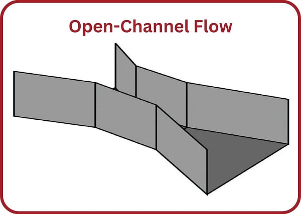
Another type of open-channel restriction used to measure liquid flow is called a flume. An illustration of a Parshall flume is shown here:
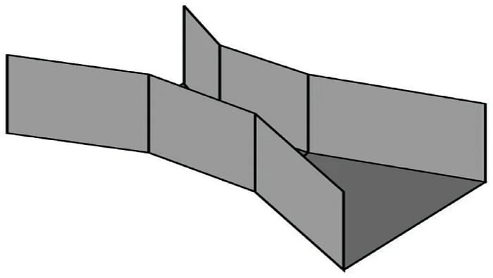
Weirs and flumes may be thought of being somewhat like “orifice plates” and “venturi tubes,” respectively, for open-channel liquid flow. Like an orifice plate, a weir or a flume generates a differential pressure that varies with the flow rate through it. However, this is where the similarities end. Exposing the fluid stream to atmospheric pressure means the differential pressure caused by the flow rate manifests itself as a difference in liquid height at different points in the channel. Thus, weirs and flumes allow the indirect measurement of liquid flow by sensing liquid height. An interesting feature of weirs and flumes is that although they are nonlinear primary sensing elements, their nonlinearity is quite different from that of an orifice.
Note the following transfer functions for different weirs and flumes, relating the rate of liquid flow through the device (\(Q\)) to the level of liquid rise upstream of the device (called “head”, or \(H\)):
\[Q = 2.48 \left( \tan {\theta \over 2} \right) H^{5 \over 2} \hspace{20pt} \hbox{V-notch weir}\]
\[Q = 3.367 L H^{3 \over 2} \hspace{20pt} \hbox{Cippoletti weir}\]
\[Q = 0.992 H^{1.547} \hspace{20pt} \hbox{3-inch wide throat Parshall flume}\]
\[Q = 3.07 H^{1.53} \hspace{20pt} \hbox{9-inch wide throat Parshall flume}\]
Where,
\(Q\) = Volumetric flow rate (cubic feet per second – CFS)
\(L\) = Width of notch crest or throat width (feet)
\(\theta\) = V-notch angle (degrees)
\(H\) = Head (feet)
It is important to note these functions provide answers for flow rate (\(Q\)) with head (\(H\)) being the independent variable. In other words, they will tell us how much liquid is flowing given a certain head. In the course of calibrating the head-measuring instruments that infer flow rate, however, it is important to know the inverse transfer function: how much head there will be for any given value of flow. Here, algebraic manipulation becomes important to the technician. For example, here is the solution for \(H\) in the function for a Cippoletti weir:
\[Q = 3.367 L H^{3 \over 2}\]
Dividing both sides of the equation by 3.367 and L:
\[{Q \over 3.367 L} = H^{3 \over 2}\]
Taking the \(\frac{3}{2}\) root of both sides:
\[\root {3 / 2} \of {Q \over 3.367 L} = H\]
This in itself may be problematic, as some hand calculators do not have an \(\root x \of y\) function. In cases such as this, it is helpful to remember that a root is nothing more than an inverse power. Therefore, we could re-write the final form of the equation using a \(2 \over 3\) power instead of a \(3 \over 2\) root:
\[\left({Q \over 3.367 L}\right)^{2 \over 3} = H\]
