Hands-on Example: Milling Machine Failure Classification Using Logistic Regression
Learn how to build a machine learning model to predict failure classification based on machine parameters using a synthetic dataset modeled after a milling machine, the same process used in real-world systems.
What is Classification and Why is it Useful?
In a previous article, I outlined the benefits of a predictive maintenance program. In this walkthrough, I aim to give a technical example of a low-budget attempt at implementing such a program for a synthetic dataset mirroring a milling machine. Classification problems in machine learning describe the use of algorithms aimed at assigning a label to a recorded example based on features of that example.
This control systems example uses a pseudo milling machine dataset that has 10,000 unique records modeling product runs. Associated with each run or record is parameter information such as process temperature, torque, and tool wear time. Within each of these records of data lies a target class; machine failure. For each data record or production run, the machine either failed (value of 1) or did not fail (value of 0). There are also categorical types of failure in further columns which can be expanded upon to explain the machine failure in greater detail.
Our goal will be to determine whether or not we can predict a milling machine failure based on the features of these runs. This task is often referred to as a binary classification problem since the prediction is limited to 2 states; fail or pass. Such a classification task can prove useful in determining which features hold more weight in machine failure.

Figure 1. Milling machine in Action. Image used courtesy of Adobe Stock
Getting Started
We will be using a Google Colab notebook for this example, which will make hardware setup seamless. The notebook is an interactive programming environment that can be shared easily amongst engineers and other data-driven professionals. These notebooks serve as a great way to perform ad-hoc data analysis while also providing an avenue for traditional control engineers to broaden their programming skills.
Furthermore, the notebook is a more powerful tool than traditional Microsoft Excel spreadsheets that litter various industries as the data analysis tool of choice. After reading Google’s “Welcome To Colaboratory” notebook that appears on initialization, open a new notebook, and we are ready to start!
To begin, download the pseudo milling machine dataset used courtesy of S. Matzka from Kaggle.com. This is a CSV file, but in order to use it for the project, it will need to be re-uploaded into the Colab workspace, using the file upload button on the left sidebar as shown below:

Data Extraction and Exploratory Data Analysis (EDA)
To get started, we will import the required modules or dependencies for the notebook in a cell and execute the cell:
# Import libraries
import pandas as pd
import numpy as np
import seaborn as sns

# Machine Learning libraries
from sklearn.linear_model import LogisticRegression
from sklearn.model_selection import train_test_split
from sklearn.preprocessing import MinMaxScaler
We will then load the required dataset from the local directory into the Google Colab environment using the code below:
# Read in milling data to a pandas DataFrame object
df = pd.read_csv('INSERT FILE PATH WITH FILENAME HERE IN QUOTES')
If you have trouble locating that file path, go back to the sidebar where the file was uploaded and retrieve the path from there.

Once loaded, preview the data by chaining the .head() method to the DataFrame object df and execute:
# Display top records of milling data
df.head()

Figure 2. DataFrame output. Image provided by author.
The head() method gives us the first 5 rows of the DataFrame. The link to the dataset describes the columns in further detail, but I will summarize some key findings and provide the associated code:
- The dataset is imbalanced, meaning that the frequency of machine failures is dwarfed by records where the machine did not fail. This can lead to model bias which will be discussed in the model evaluation section. For now, understand that this is a real-world challenge in implementing defect detection in manufacturing. It is also present in other industries, such as fraud detection in finance.

Figure 3. Imbalanced Machine Failure dataset. Image supplied by author
- The “UDI” and “Product ID” fields serve as a clustered primary key in that for each record, they are unique. This prevents us from extracting any meaningful correlation from these fields since they are no different than an index:

Figure 4. Product ID and UDI fields are unique keys. Image provided by author
- As any manufacturing engineer would understand, wear time is likely to correlate to failure. Drilling down within failure records yields an increased frequency in failures with greater wear time clustered around 200 minutes:
Figure 5. Failure frequency distributed around 200 minutes of tool wear. Image provided by author.
Preprocessing
To build a machine learning model, DataFrames must be preprocessed.
The steps outlined here are only a barebones framework to maintain brevity of article scope.
The “Product ID” and “UDI” fields will be dropped since they are redundant to the index:
df.drop(['Product ID','UDI'], axis = 1, inplace = True)
Any null values will need to be imputed or dropped from the DataFrame. In this example, there are no null values in any fields. This is not reflective of the real world, as missing data is common:

Figure 6. Mean of null values per column. Image provided by author.
Machine learning models function in terms of numbers. Therefore, categorical string data in the “Type” column must be broken into 3 separate columns of dummy variables (0 or 1s):
# Create dummy variables from type column to dataframe
type_dummies = pd.get_dummies(df['Type'].apply(pd.Series).stack()).sum(level=0)
# Join dummy variables on index of original dataframe
df2 = df.join(other = type_dummies)
df2.drop(columns = ['Type'], inplace = True)
df2.head()
Please note the “L”, “M”, “H” columns on the end, and removal of the “Type” column:

Figure 7. Dummy columns of Type field added to DataFrame. Image provided by author.
Before beginning the model build and evaluation, a crude check of Pearson correlation can be performed on the attributes of the DataFrame. Torque and Tool wear appear to be correlated to the Machine failure target most closely:
# High correlation of failure to torque and tool wear
sns.heatmap(df2.corr());

Figure 8. Pearson’s correlation heatmap of attribute to attribute in DataFrame. Image provided by author.
Model Build and Evaluation
The model build will use a logistic regression model to classify the Machine failure field. Logistic regression is used in binary classification since the target field is either a 0 or a 1 (discrete). Some techniques that are being used in the example include:
- Oversampling: Replicating existing examples of the machine failure records to match the number of machine not fail records. Attempts to balance dataset.
- Scaling: The independent variables fed to the model are scaled on a scale of 0 to 1. For example, rotational speed values in the dataset are much greater than other parameters. This could inaccurately weight rotational speed heavier than other parameters. Therefore, all parameters are scaled on a scale of 0 to 1.
Model code below:
# Separate target from independent variables
independent_vars = df2.drop(['Machine failure','TWF','HDF','PWF','OSF','RNF'], axis = 1)
target = df2['Machine failure']
X = independent_vars
y = target

# Split data into training and testing data
X_train, X_test, y_train, y_test = train_test_split(X, y, test_size=0.2, random_state=None)

# Oversample the minority class; mill machine failures
oversampler = RandomOverSampler(sampling_strategy = 'minority')

# Apply oversampling to the training data
X_train, y_train = oversampler.fit_resample(X_train, y_train)

# Fit the scaler on both the training and testing data for independent variables
scaler = MinMaxScaler()
X_train = scaler.fit_transform(X_train)
X_test = scaler.transform(X_test)

# Create the logistic regression model and fit on the training data
modelOversample = LogisticRegression()
modelOversample.fit(X_train, y_train)

# Accuracy
score_test = modelOversample.score(X_test, y_test)
score_train = modelOversample.score(X_train, y_train)
print(f"Accuracy on test data: {score_test*100}%")
print(f"Accuracy on train data: {score_train*100}%")

Accuracy on test data: 81.25%
Accuracy on train data: 82.07217694994179%
Since oversampling was implemented, an accuracy metric can be used. This metric shows that our model correctly predicted the machine failure target 81.25% of the time. Not bad, but not great either. This model serves more as an introduction to the concept of logistic regression in industrial controls application, and there is ample opportunity for improvement.
Real World Conclusion
I’m going to pose the logical progression of this project in a situational-based scenario as if you were at a company that is just starting to explore predictive maintenance.
You’ve made it through collecting data reliably, processing the data, and building out a rough logistic regression model based on the data. You’ve overcome many technical hurdles and it’s taken longer than you, your boss, or team anticipated. Before proceeding further, you meet with the stakeholders and leadership to share the solution you have thus far. In the meeting, you will likely encounter the following questions:
- The model helps highlight which parameters have a greater influence on predicting a failure. However, if we push our milling machine's parameters to the USL or LSL or outside of production qualified parameter limits we shouldn’t be surprised at the increased probability of machine failure. What value does this model bring?
- Can we predict more specifically which type of failure can occur?
- Can we predict the tool's wear time to failure?
- When can we have the front-end application of the model, so that technicians can input new parameters to test whether the machine will fail?
These are all valid questions that can be explored in future articles. The reason I present this article and the further questions, however, is to show that predictive maintenance is difficult to implement. It’s a complex, multi-faceted system that requires strategy and resources to build and maintain.
Many high-level articles gloss over the technical breadth and challenges that will be faced by various companies in implementing these systems. The false perception that the “lights-out” smart factory is achievable in unrealistic timelines abounds because the details are not well understood. With that being said, these systems are not impossible to implement.
With the right team, resources, management, or vendor/partner, it is achievable. The devil is certainly in the details when it comes to predictive maintenance systems.


