Huffman Coding for Data Compression

It is often desirable to reduce the amount of storage required for data. In general, it is an advantage to do this for cost and/or performance reasons when storing data on media, such as a hard drive, or transmitting it over a communications network. Since Huffman coding is a lossless data compression algorithm, the original data will always be perfectly restructured from the compressed data.

Suppose we would like to encode the following phrase:

 

 

One way to do that would be to represent each symbol as a unique pattern of bits. Since there are nine distinct symbols (including the space, which we’ll represent as an underscore “_”), each symbol can be represented by a bit pattern. A fixed-length pattern of four bits can represent 16 distinct symbols, so our nine symbols can be represented as follows:

 

Symbol	Bit Pattern (code)	Number of Occurrence
C	0000	1
A	0001	1
L	0010	6
_	0011	3
M	0100	2
E	0101	3
O	0110	2
W	0111	2
F	1000	1

Figure 1. Fixed-length pattern and symbols.

 

Note that the total number of symbols in the above phrase is 21; therefore, a 4-bit code representing each symbol requires 84 bits. But can we do better than that?

Typically, applying Huffman coding to the problem should help, especially for longer symbol sequences. Huffman coding takes into consideration the number of occurrences (frequency) of each symbol. Applying the algorithm results in a variable-length code where shorter-length codes are assigned to more frequently appearing symbols. 

The resulting code obeys the “prefix property,” meaning no other code appears as the initial string of symbols in some other code. For example, no home phone number begins with the “911,” as that creates an obvious problem. As we will see, the prefix property is enforced by the idea that the code is represented by a binary tree where the symbols appear only at the leaf nodes.

 

The Huffman Algorithm

We begin by sorting the list of symbols, according to their frequency, in ascending order (figure 2).

Symbol(s)	Frequency of Occurrence
C	1
A	1
F	1
M	2
O	2
W	2
E	3
_	3
L	6

Figure 2. List of symbols, according to frequency, in ascending order.

 

Elements from this initial list will be both removed and added. This list builds a binary tree that defines our code. When removing elements from the list, the two elements with the smallest frequency are removed first. This will always be the first two rows. 

We begin by removing both the C and A symbols and forming a binary tree. Note that we label the parent node as the concatenation of symbols of its two child nodes. The number in parenthesis represents the frequency of occurrence of the symbol. The parent node can be interpreted as, “the frequency of occurrence of either a C or an A is 2," which is simply the sum of its child occurrences.

 

Step 1

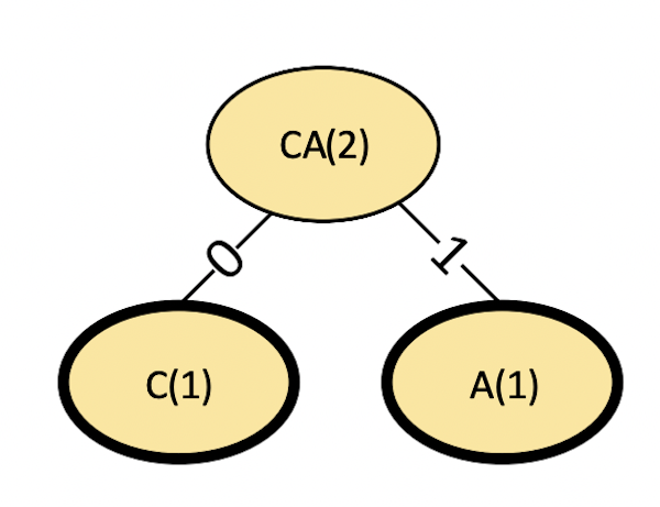
Figure 3. Step 1 in a Huffman code.

 

Also, by convention, the left branch is labeled 0, and the right branch is labeled 1. Since we created a new node named “CA,” we must insert this into our table. New nodes are always inserted to maintain the sorted order of the table. Figure 4 shows the revised table after removing C and A and inserting CA.

 

Symbol(s)	Frequency of Occurrence
F	1
CA	2
M	2
O	2
W	2
E	3
_	3
L	6

Figure 4. Updated symbols list.

 

Continuing, we add F since it is a new node. It is paired with the existing node CA, which we added in the last step, and the new parent FCA is added.

 

Step 2

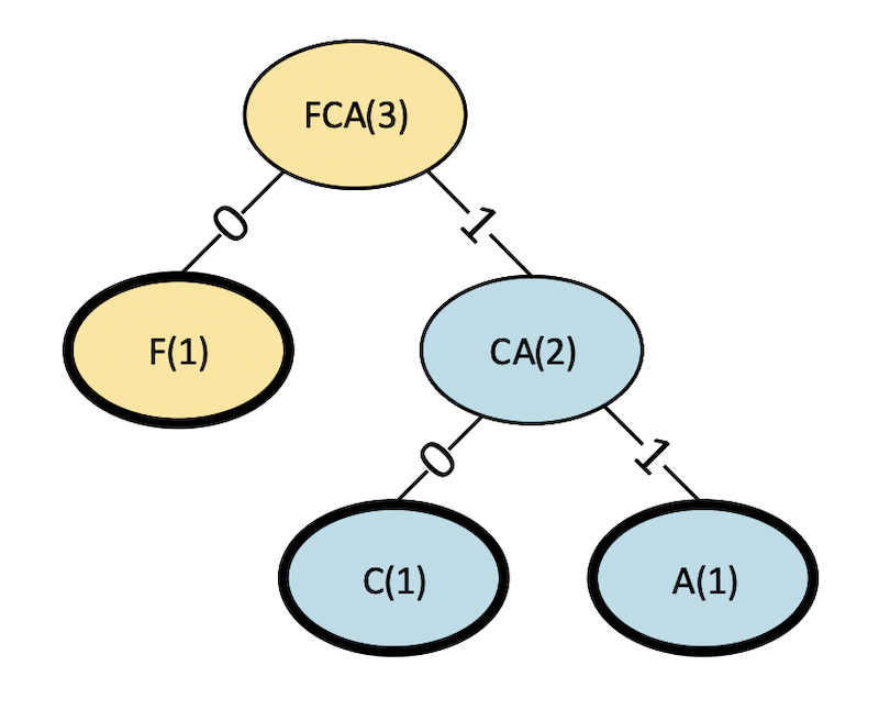
Figure 5. Step 2 in a Huffman code.

 

The revised table is as follows.

 

Symbol(s)	Frequency of Occurrence
M	2
O	2
W	2
FCA	3
E	3
_	3
L	6

Figure 6. Revised table after removing F and CA, and adding FCA.

 

We then repeat this process until the table is empty.

 

Step 3

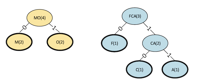
Figure 7. Step 3 binary tree in a Huffman code.

 

Symbol(s)	Frequency of Occurrence
W	2
FCA	3
E	3
_	3
MO	4
L	6

Figure 8. Revised table for step 3.

 

Step 4

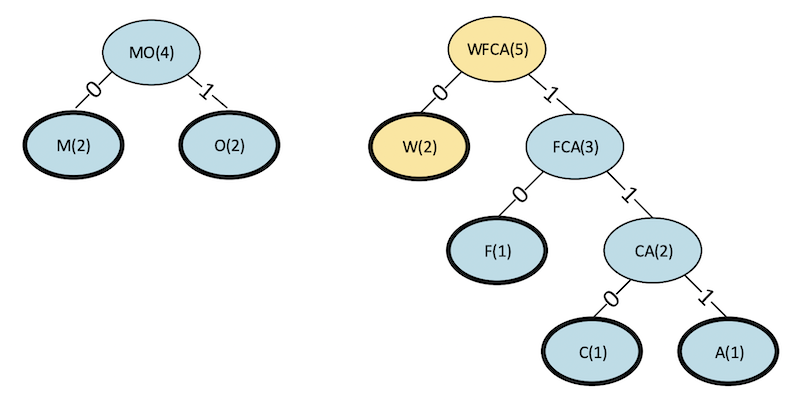
Figure 9. Step 4 binary tree for a Huffman code.

 

Symbol(s)	Frequency of Occurrence
E	3
_	3
MO	4
WFCA	5
L	6

Figure 10. Revised table for step 4.

 

Step 5

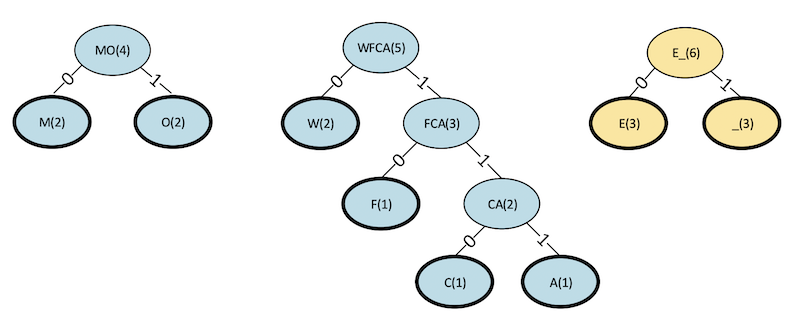
Figure 11. Step 5 binary tree for a Huffman code.

 

Symbol(s)	Frequency of Occurrence
MO	4
WFCA	5
E_	6
L	6

Figure 12. Revised table for step 5.

 

Step 6

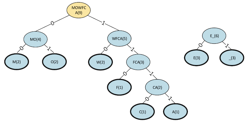
Figure 13. Step 6 binary tree for a Huffman code.

 

Symbol(s)	Frequency of Occurrence
E_	6
L	6
MOWFCA	9

Figure 14. Revised table for step 6, after removing MO and WFCA, and adding MOWFCA.

 

Step 7

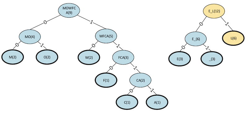
Figure 15. Step 7 binary tree for a Huffman code.

 

Symbol(s)	Frequency of Occurrence
MOWFCA	9
E_L	12

Figure 16. Revised table for step 7, after removing E_ and L, and adding E_L.

 

Step 8 (Final)

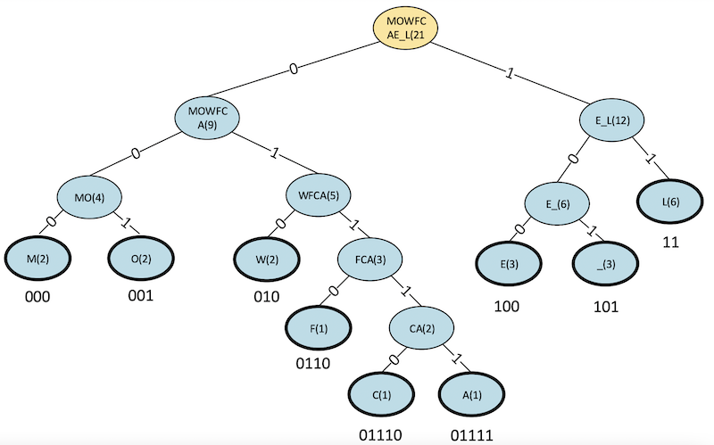
Figure 17. Step 8 (final) binary tree for a Huffman code.

 

Our table is now empty, and our binary tree is complete. Note that the Huffman codes for each symbol have been added.

 

Huffman Code Results

In our completed tree, all of the symbols appear as leaf nodes (with bold outlines). Codes have been assigned by starting at the root node and recording the 0/1 sequence down the path, which leads to the particular symbol. For example, the code for E is obtained, as shown in figure 18.

 

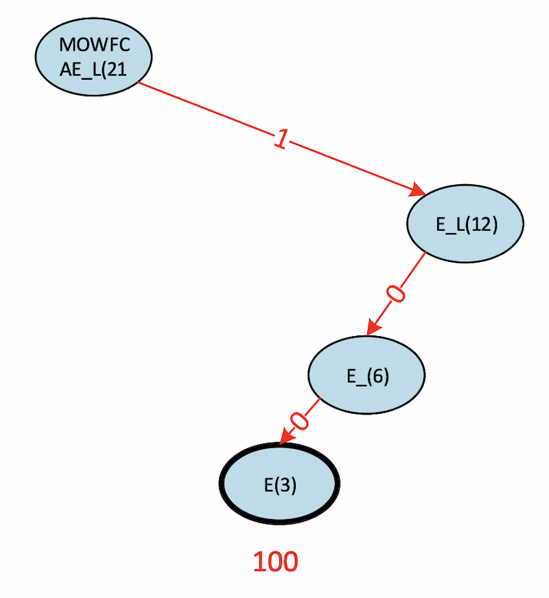
Figure 18. Binary tree for obtaining the code for E.

 

Symbol	Bit Pattern (code)	Number of Occurrences	Number of Bits in Code	Total Bits Used by the Symbol
C	01110	1	5	5
A	01111	1	5	5
L	11	6	2	12
_	101	3	3	9
M	000	2	3	6
E	100	3	3	9
O	001	2	3	6
W	010	2	3	6
F	0110	1	4	4

Figure 19. A summary of our Huffman code.

 

Note in figure 19 that the last column is simply the product of the two previous columns.

Also, notice the symbols that appear more frequently tend to have fewer bits in their code. This behavior is the essence of the Huffman algorithm.

So, our Huffman encoding of our original phrase:

 

 

Becomes:

 

 

(Commas added for clarity only).

Only 62 total bits to encode our original string. Recall that our original 4-bit fixed-length code required 84 bits, representing a data compression of 26%.

To decode our phrase (commas removed below):

 

 

We begin at the root of the tree and follow the path indicated by the binary digits until we reach a leaf node. As you can see below, this results in the first letter of our phrase, a “C.” We then repeat the process continuing from where we left off until we have no more bits to process.

 

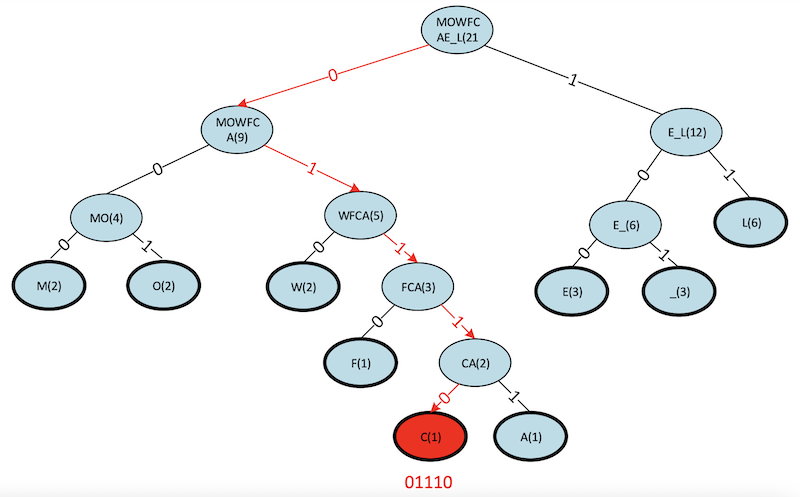
Figure 20. The final Huffman algorithm showing the first letter, “C.”

 

We have seen how the Huffman coding algorithm works and observed its inherent simplicity and effectiveness. In practice, Huffman coding is widely used in many applications. For example, it is used in "ZIP" style file compression formats, *.jpeg and *.png image formats, and *.mp3 audio files.