Utilizing Mapping and Localization in SLAM for Robotics

SLAM stands for simultaneous localization and mapping. So, clearly, localization and mapping are key. This article elaborates on robot mapping and localization, the mathematical representation of the SLAM problem, and creates a precursor for the final article in this introductory series that explains the algorithms and techniques used in the industry.

This article is part of a larger series introducing SLAM. The previous article provided an overview of mobile robots and the types of SLAM applicable to them. If you are new to the concept of SLAM, it is highly recommended you read that article first. 

 

 

 

 

 

 

 

Why Mapping and Localization are Crucial to SLAM

SLAM is essentially a chicken-and-egg problem. An accurate map can only be created and augmented when the robot knows its own location within it, while accurate robot pose is dependent on the precision of generated maps.

Mapping is the process of creating a desired computational representation of the environment: the terrain, objects, humans, and vegetation. Maps are used to inform the robot about feasible areas of motion in the environment and definition of the spatial models of the objects in the scene.

Localization refers to determining the pose of the robot in the map. Pose is comprised of the 3D Cartesian position \(\left (x ,y ,z \right )\) and orientation (quaternion \(\left [q_w, q_x, q_y, q_z \right ]\) or Euler \(\left [\alpha , \beta, \gamma \right ]\)) of the robot with respect to the origin of the derived map. Accurate robot pose estimation is critical to all frame-based vector measurements made from RADAR, LiDAR, depth camera, and sensors.

Since mapping and localization can potentially use the same sensors, the process is susceptible to bias and cascading inaccuracies in the information handling and processing steps.

 

Robot Mapping

Intuitive representations of maps are only useful for humans, so robots/computers need programmatic representations using certain programming data structures. They could be represented as weighted and directed graphs, adjacency matrices, or linked lists. Camera-generated feature graphs have more information to be stored and are defined in custom data structures.

The simplest computational representation of the different world objects for static 3D maps is done as coarse bounding boxes with predefined locations. These most common bounding box representations are axis-aligned bounding boxes (AABB) and oriented bounding boxes (OBB). These are rudimentary representations only meant for discrete object scenes and thus not very extensible to dynamic SLAM applications. However, they can be a starter.

Robot mapping is a complex process and map representations depend on the type of objects from the environment to be included in the map. SLAM maps are usually 2D and 3D for terrestrial and aerial robots, respectively. Wheeled mobile robot navigation is limited to 2D terrain and thus maps are only defined for 2D, while 3D scene interpretation is only meant for obstacle avoidance. The 3D objects are projected onto one plane to create 2D maps for mobile robots. There are two broad categories of maps: metric and topological.

 

Metric Maps

Metric maps represent an environment’s known bounds with appropriate edges, area, and locations of the free and occupied configuration space. This is a geometric representation of the robot environment analogous to a political map of any country with cities and states and their boundaries and distances. 

Occupancy grids are the standard but coarse, metric map representations are used in SLAM and robotics. Occupancy grids break the complete map into smaller grids of desired dimensions. Each cell is associated with a probability of the cell being occupied by an obstacle or free for the robot’s motion in the corresponding real-world area. Occupancy grids may be 2D or 3D depending on the type of robot navigation (terrestrial or aerial).

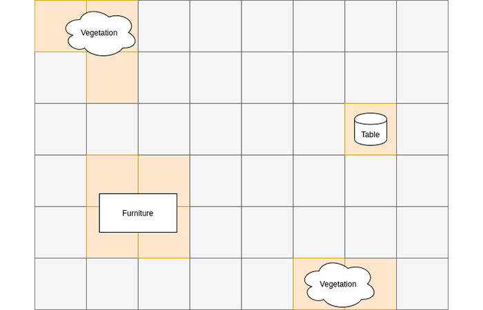
Figure 1. A sample occupancy grid. Pink cells are occupied and blue cells are free.

 

Most global planners used to plan robot motion for long distances in the map use OGs represented as graphs and implement common search algorithms like A*, Djikstra, and their variants motion planners.

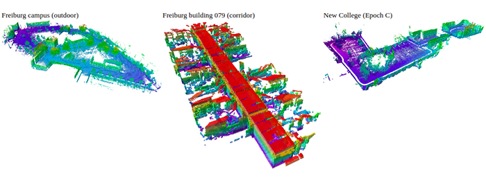
Figure 2. 3D Occupancy grids generated by Octomap (Image Source: Octomap Website).

 

Topological Maps

Topological maps store information about distinct landmarks like walls, edges, vegetation, lane boundaries, and more physical features in the environment. Topological maps are analogous to the physical maps of the world with markings for natural elements like rivers and mountains. 

Feature maps are typical topological maps used in robotics with certain marks representing the point landmarks obtained. Feature maps have vivid information about permissible areas of robot motion and thus help it navigate safely without collision. 

 

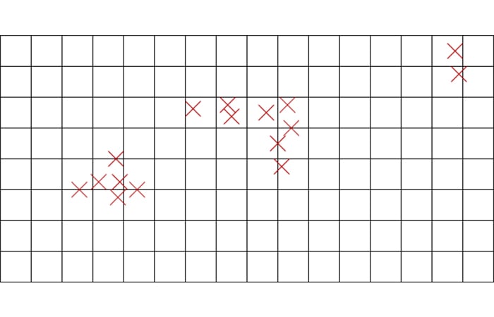
Figure 3. Feature map (X represents a landmark point).

 

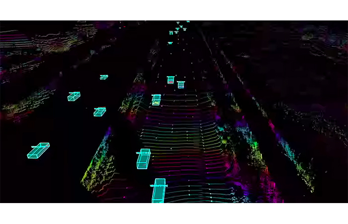
Figure 4. High-definition map for self-driving applications (Image Source: Luminar Technology Website)

 

Depth cameras and laser scanners are the most important sensors for creating and updating maps. When the robot is exploring the world, it keeps appending elements and navigable/obstructed regions of the map based on the observations using several algorithms explained in the next part of this series. Often, the robot closes the loop when it re-encounters previously seen regions of the scene and updates the complete map to accommodate for errors that were derived based on previous encounters.

Robot Localization

Determining the pose of the robot is the most important step of SLAM, as every observation, control loop action, and estimate depends on the robot’s location. The various inaccuracies in the system are capable of causing serious variations in the robot pose estimation which cascades to mapping and back. Consistent with other aspects, the robot pose is also a probabilistic representation whose variance tends to explode in a very short time unless sensor fusion and learning techniques are deployed. 

Sensor measurement-based odometry (obtained from IMUs, encoders, or both), combined with external measurements from range finders or cameras, obtains a probabilistic estimate of the robot pose. Very often, visual odometry is also used in this process. Academic research has been done on using deep learning techniques for visual odometry estimation. 

 

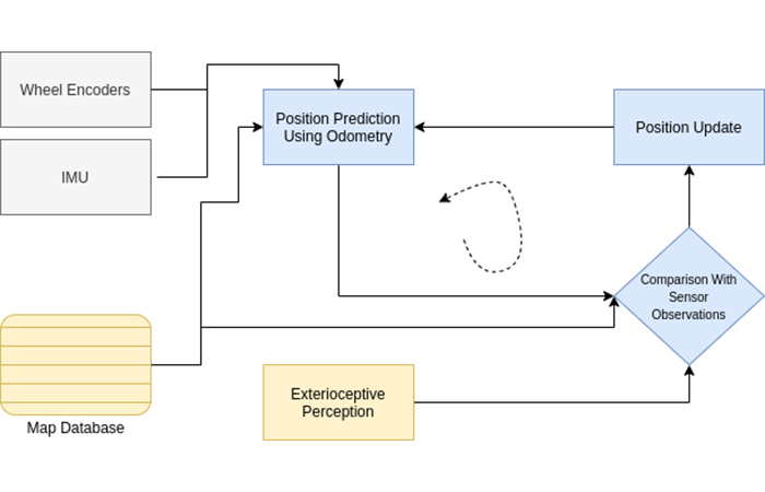
Figure 5. A sample localization pipeline.

 

Robot localization is tricky as there are significant communication and data processing delays that make sensor data obsolete to the position and time observation. Thus, there are several synchronization techniques used for sensor information sanity checks as well as several frame transformations to avoid incorrect data measurements.

Absolute pose estimation defines the robot pose in the global frame while the map is still being built as the robot explores. On a lot of occasions, one certain loop closure can change the shape of a significant portion of the map. Thus, relative pose estimation derives robot pose relative to a previous landmark or previous robot pose, making it more feasible and less prone to accumulation errors or cascading effects. 

 

The Mathematical Formulation for SLAM 

The standard mathematical representation of a SLAM problem states:

Given the robot control input(u), sensor observations(z), prior information about the environment map(m), and robot pose(x) determine the updated values of m and x. 

The pose and map could be sequences or a snapshot depending on the type of application. 

Additional tasks include iterative updates to older values for m and x as the robot navigates through the same locations and scenes.

 

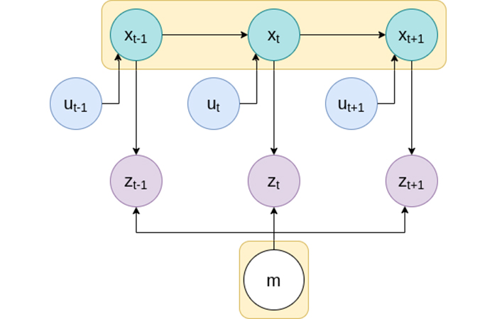
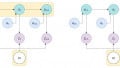
Figure 6. The SLAM problem: obtain the pose x and map m 

 

The mathematical formulation of the SLAM problem is:

\[p(x_{1:t},m | z_{1:t} ,u_{0:t-1}) = p(x_{1:t}|z_{1:t},u_{0:t-1})* p(m|x_{1:t},z_{1:t})\]

\(p(x|z)\) is the probability of an \(x\) given \(z\) and \(z_{1:t} = {z_1, z_2,... z_{t-11}, z_{t-2}}\)

For any mobile robot navigation, the control input \(u\) defines the intent for the motion of the robot, which the robot may or may not be able to implement completely due to various hardware and software limitations. The robot pose at any time can be mathematically represented as a function of the pose at the previous timestamp and the control input. This is called the motion model, and it’s mathematical formulation is:

\[x_t =f( x_{t-1}, u_t )\]

 

The motion model uses the kinematic model mentioned in the previous article and is the prediction step for any localization efforts.

The various observations made by the sensors depend on the robot’s current pose within the map and the latest map. This mathematical representation is called the observation model.  The robot pose is used to transform relative geometric measurements for distances and obstacles to the robot or the map origin frame. The observation model formulation is:

\[z_t =f( x_t,m )\]

 

Intuitively, this represents that a rangefinder’s distance and bearing measurement can only be reflected on the map depending on where the robot is in the map, and what the map actually looks like.

This formulation defines the computation of the list of the robot’s poses from the start of time and derives the complete map of the robot, given posterior robot pose information (based on observations and control input) and the posterior map information (based on pose and observations).

 

Review of Key Points and Next Steps

This article explains what robot localization and mapping comprises and how sensors contribute towards their implementation. The programmatic representation of the problem paves the way for its implementation.

The appropriate next step is to learn the common algorithms required to implement SLAM using programming languages C++ or Python. There are several other intermediary data manipulation, sensor data processing, data transfer, and architectural aspects of implementing SLAM.