 Facebook
 Google
 GitHub
 Linkedin
What is Hydrostatic Pressure?
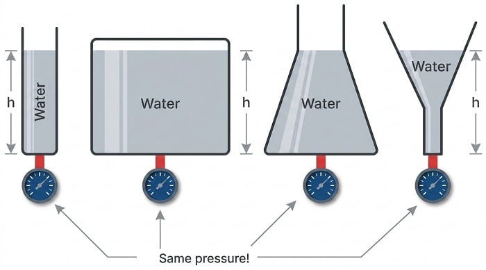
A vertical column of fluid generates a pressure at the bottom of the column owing to the action of gravity on that fluid. The greater the vertical height of the fluid, the greater the pressure, all other factors being equal. This principle allows us to infer the level (height) of liquid in a vessel by pressure measurement.
Pressure of a Fluid Column
A vertical column of fluid exerts a pressure due to the column’s weight. The relationship between column height and fluid pressure at the bottom of the column is constant for any particular fluid (density) regardless of vessel width or shape.
This principle makes it possible to infer the height of liquid in a vessel by measuring the pressure generated at the bottom:
The mathematical relationship between liquid column height and pressure is as follows:
\[P = \rho g h \hskip 100pt P = \gamma h\]
Where,
\(P\) = Hydrostatic pressure
\(\rho\) = Mass density of fluid in kilograms per cubic meter (metric) or slugs per cubic foot (British)
\(g\) = Acceleration of gravity
\(\gamma\) = Weight density of fluid in newtons per cubic meter (metric) or pounds per cubic foot (British)
\(h\) = Height of vertical fluid column above point of pressure measurement
For example, the pressure generated by a column of oil 12 feet high (\(h\)) having a weight density of 40 pounds per cubic foot (\(\gamma\)) is:
\[P = \gamma h\]
\[P_{oil} = \left({40 \hbox{ lb} \over \hbox{ft}^3 }\right) \left({12 \hbox{ ft} \over 1}\right) = {480 \hbox{ lb} \over \hbox{ft}^2 }\]
Note the cancellation of units, resulting in a pressure value of 480 pounds per square foot (PSF). To convert into the more common pressure unit of pounds per square inch, we may multiply by the proportion of square feet to square inches, eliminating the unit of square feet by cancellation and leaving square inches in the denominator:
\[P_{oil} = \left({480 \hbox{ lb} \over \hbox{ft}^2 }\right) \left({1^2 \hbox{ ft}^2 \over 12^2 \hbox{ in}^2 }\right)\]
\[P_{oil} = \left({480 \hbox{ lb} \over \hbox{ft}^2 }\right) \left({1 \hbox{ ft}^2 \over 144 \hbox{ in}^2 }\right)\]
\[P_{oil} = {3.33 \hbox{ lb} \over \hbox{in}^2 } = 3.33 \hbox{ PSI}\]
Thus, a pressure gauge attached to the bottom of the vessel holding a 12 foot column of this oil would register \(3.33\) PSI. It is possible to customize the scale on the gauge to read directly in feet of oil (height) instead of PSI, for convenience of the operator who must periodically read the gauge. Since the mathematical relationship between oil height and pressure is both linear and direct, the gauge’s indication will always be proportional to height.
An alternative method for calculating pressure generated by a liquid column is to relate it to the pressure generated by an equivalent column of water, resulting in a pressure expressed in units of inches of water column ("W.C.) which may then be converted into PSI or any other unit desired.
For our hypothetical 12-foot column of oil, we would begin this way by calculating the specific gravity (i.e. how dense the oil is compared to water). With a stated weight density of 40 pounds per cubic foot, the specific gravity calculation looks like this:
\[\hbox{Specific Gravity of oil} = {\gamma_{oil} \over \gamma_{water}}\]
\[\hbox{Specific Gravity of oil} = {40 \hbox{ lb/ft}^3 \over 62.4 \hbox{ lb/ft}^3}\]
\[\hbox{Specific Gravity of oil} = 0.641\]
The hydrostatic pressure generated by a column of water 12 feet high, of course, would be 144 inches of water column (144 "W.C.). Since we are dealing with an oil having a specific gravity of 0.641 instead of water, the pressure generated by the 12 foot column of oil will be only 0.641 times (64.1%) that of a 12 foot column of water, or:
\[P_{oil} = (P_{water})(\hbox{Specific Gravity})\]
\[P_{oil} = (144 \hbox{ "W.C.})(0.641)\]
\[P_{oil} = 92.3 \hbox{ "W.C.}\]
We may convert this pressure value into units of PSI simply by dividing by 27.68, since we know 27.68 inches of water column is equivalent to 1 PSI:
\[P_{oil} = \left({92.3 \hbox{ "W.C.} \over 1}\right) \left({1 \hbox{ PSI} \over 27.68 \hbox{ "W.C.}}\right)\]
\[P_{oil} = 3.33 \hbox{ PSI}\]
As you can see, we arrive at the same result as when we applied the \(P = \gamma h\) formula. Any difference in value between the two methods is due to imprecision of the conversion factors used (e.g. 27.68 "W.C., 62.4 lb/ft\(^{3}\) density for water).
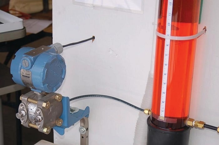
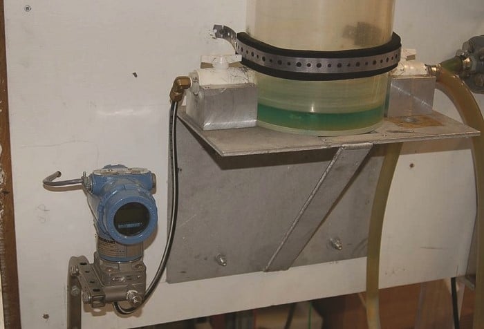
Any type of pressure-sensing instrument may be used as a liquid level transmitter by means of this principle. In the following photograph, you see a Rosemount model 1151 pressure transmitter being used to measure the height of colored water inside a clear plastic tube:
In most level-measurement applications, we are concerned with knowing the volume of the liquid contained within a vessel, and we infer this volume by using instruments to sense the height of the fluid column. So long as the vessel’s cross-sectional area is constant throughout its height, liquid height will be directly proportional to stored liquid volume. Pressure measured at the bottom of a vessel can give us a proportional indication of liquid height if and only if the density of that liquid is known and constant. This means liquid density is a critically important factor for volumetric measurement when using hydrostatic pressure-sensing instruments. If liquid density is subject to random change, the accuracy of any hydrostatic pressure-based level or volume instrument will be correspondingly unreliable.
It should be noted, though, that changes in liquid density will have absolutely no effect on hydrostatic measurement of liquid mass, so long as the vessel has a constant cross-sectional area throughout its entire height. A simple thought experiment proves this: imagine a vessel partially full of liquid, with a pressure transmitter attached to the bottom to measure hydrostatic pressure. Now imagine the temperature of that liquid increasing, such that its volume expands and has a lower density than before. Assuming no addition or loss of liquid to or from the vessel, any increase in liquid level will be strictly due to volume expansion (density decrease). Liquid level inside this vessel will rise, but the transmitter will sense the exact same hydrostatic pressure as before, since the rise in level is precisely countered by the decrease in density (if \(h\) increases by the same factor that \(\gamma\) decreases, then \(P = \gamma h\) must remain the same!). In other words, hydrostatic pressure is seen to be directly proportional to the amount of liquid mass contained within the vessel, regardless of changes in liquid density. This is useful to know in applications where true mass measurement of a liquid (rather than volume measurement) is either preferable or necessary.
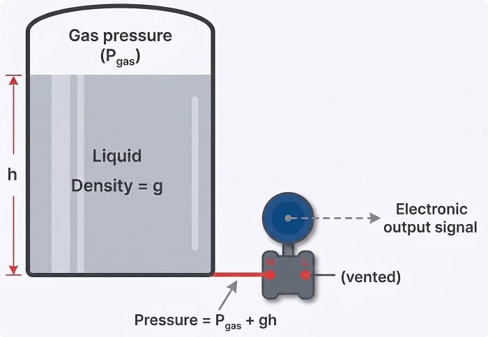
Differential pressure transmitters are the most common pressure-sensing device used in this capacity to infer liquid level within a vessel. In the hypothetical case of the oil vessel just considered, the transmitter would connect to the vessel in this manner (with the high side toward the process and the low side vented to atmosphere):
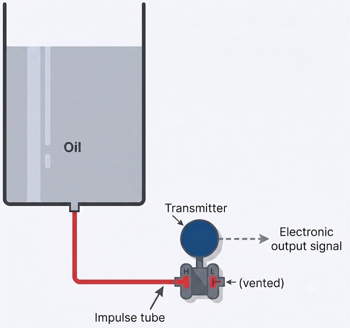
Connected as such, the differential pressure transmitter functions as a gauge pressure transmitter, responding to hydrostatic pressure exceeding ambient (atmospheric) pressure. As liquid level increases, the hydrostatic pressure applied to the “high” side of the differential pressure transmitter also increases, driving the transmitter’s output signal higher.
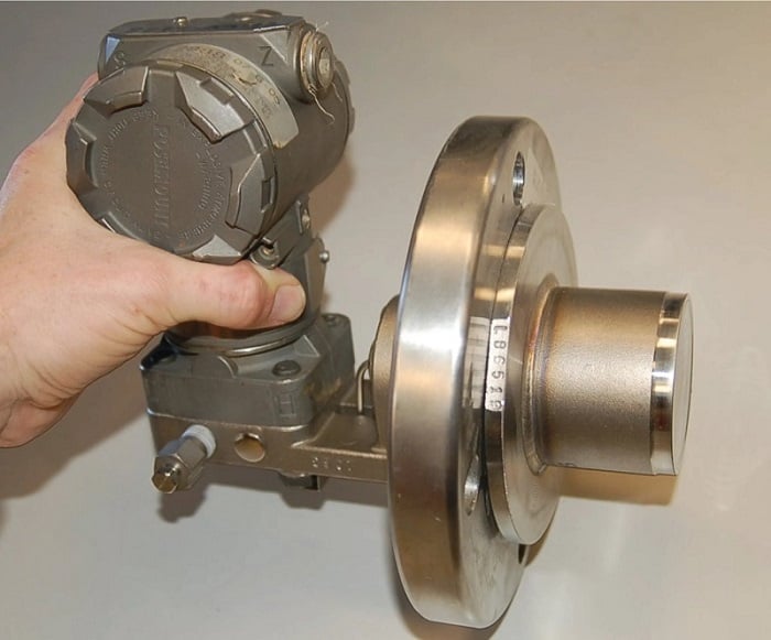
Some pressure-sensing instruments are built specifically for hydrostatic measurement of liquid level in vessels, eliminating with impulse tubing altogether in favor of a special kind of sealing diaphragm extending slightly into the vessel through a flanged pipe entry (commonly called a nozzle). A Rosemount hydrostatic level transmitter with an extended diaphragm is shown here:
The calibration table for a transmitter close-coupled to the bottom of an oil storage tank would be as follows, assuming a zero to twelve foot measurement range for oil height, an oil density of 40 pounds per cubic foot, and a 4-20 mA transmitter output signal range:
| Oil level | Percent of Range | Hydrostatic Pressure | Transmitter Output |
|---|---|---|---|
| 0 ft | 0 % | 0 PSI | 4 mA |
| 3 ft | 25 % | 0.833 PSI | 8 mA |
| 6 ft | 50 % | 1.67 PSI | 12 mA |
| 9 ft | 75 % | 2.50 PSI | 16 mA |
| 12 ft | 100 % | 3.33 PSI | 20 mA |
Bubbler Systems
An interesting variation on this theme of direct hydrostatic pressure measurement is the use of a purge gas to measure hydrostatic pressure in a liquid-containing vessel. This eliminates the need for direct contact of the process liquid against the pressure-sensing element, which can be advantageous if the process liquid is corrosive.
Such systems are often called bubble tube or dip tube systems, the former name being appropriately descriptive for the way purge gas bubbles out the end of the tube as it is submerged in process liquid. A very simple bubbler system may be simulated by gently blowing air through a straw into a glass of water, maintaining a steady rate of bubbles exiting the straw while changing the depth of the straw’s end in the water:
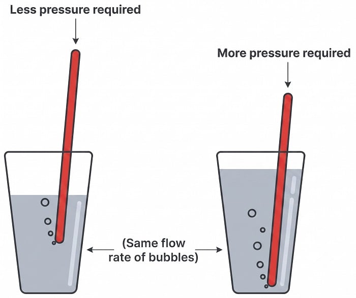
The deeper you submerge the straw, the harder it becomes to blow bubbles out the end with your breath. The hydrostatic pressure of the water at the straw’s tip becomes translated into air pressure in your mouth as you blow, since the air pressure must just exceed the water’s pressure in order to escape out the end of the straw. So long as the flow rate of air is modest (no more than a few bubbles per second), the air pressure will be very nearly equal to the water pressure, allowing measurement of water pressure (and therefore water depth) at any point along the length of the air tube.
If we lengthen the straw and measure pressure at all points throughout its length, it will be the same as the pressure at the submerged tip of the straw (assuming negligible friction between the moving air molecules and the straw’s interior walls):
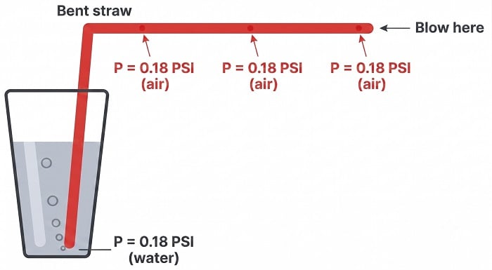
This is how industrial “bubbler” level measurement systems work: a purge gas is slowly introduced into a “dip tube” submerged in the process liquid, so that no more than a few bubbles per second of gas emerge from the tube’s end. Gas pressure inside all points of the tubing system will (very nearly) equal the hydrostatic pressure of the liquid at the tube’s submerged end. Any pressure-measuring device tapped anywhere along the length of this tubing system will sense this pressure and be able to infer the depth of the liquid in the process vessel without having to directly contact the process liquid.
Bubbler-style liquid level measurement systems are especially useful when the process liquid in question is highly corrosive, prone to plugging sample ports, or in any other way objectionable to have in direct contact with a pressure sensor. Unlike pressure sensors which must use diaphragms or other flexible (usually metallic) sensing elements and therefore may only be constructed from a limited range of materials, a dip tube need not be flexible and therefore may be constructed of any material capable of withstanding the process liquid. A process liquid so corrosive that non-metallic vessels are required to hold it would preclude direct contact with a metal pressure gauge or pressure transmitter, but would be easily measured with a bubbler system provided the dip tube were made out of plastic, ceramic, or some other material immune to corrosion. A process liquid so laden with solids that it plugs up any non-flowing port would preclude pressure measurement via a sample port and impulse line, but would be easily measured by a bubbler system where the dip tube is continuously purged with clean gas. Level measurement applications where direct contact with the pressure sensor would render access to that sensor inconvenient or even impossible are made much more practical by using a bubbler system, where the pressure sensor may be located anywhere along the dip tube’s length and therefore easily located where maintenance personnel can access it.
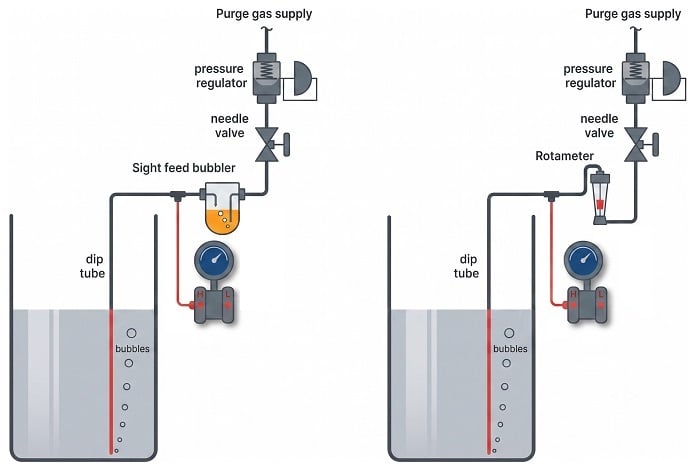
Excessive purge gas flow through the tube will result in additional pressure caused by frictional pressure drop along the tube’s length, causing the pressure-sensing instrument to falsely register high. A key detail of any practical bubble tube system, therefore, is some means to monitor and control gas flow through the tube. A common construction uses either a rotameter or a sightfeed bubbler to monitor purge gas flow rate, with a needle valve to restrict that flow:
A more sophisticated solution to the problem of purge gas flow rate is to install a flow-regulator in lieu of a pressure regulator and needle valve, a mechanism designed to automatically monitor and throttle gas flow to maintain a constant purge rate. Flow regulators compensate for changes in dip tube pressure and in gas supply pressure, eliminating the need for a human operator to periodically adjust a needle valve.
Limiting the flow of purge gas is also important if that purge gas is expensive to obtain. For bottled gases such as nitrogen (necessary in processes requiring a non-reactive purge), the cost of purchasing tanks of compressed gas is obvious. For air-purged systems the cost is still present, but not so obvious: the cost of running an air compressor to maintain continuous purge air pressure. Either way, limiting the flow rate of purge gas in a bubbler system yields economic benefits aside from increased measurement accuracy.
As with all purged systems, certain criteria must be met for successful operation. Listed here are some of them:
- The purge gas supply must be reliable: if the flow stops for any reason, the level measurement will cease to be accurate, and the dip tube may even plug with debris!
- The purge gas supply pressure must exceed the hydrostatic pressure at all times, or else the level measurement range will fall below the actual liquid level.
- The purge gas flow must be maintained at a low rate, to avoid pressure drop errors (i.e. excess pressure measured due to friction of the purge gas through the tube).
- The purge gas must not adversely react with the process.
- The purge gas must not contaminate the process.
- The purge gas must be reasonable in cost, since it will be continuously consumed over time.
One measurement artifact of a bubble tube system is a slight variation in pressure each time a new bubble breaks away from the end of the tube. The amount of pressure variation is approximately equal to the hydrostatic pressure of process fluid at a height equal to the diameter of the bubble, which in turn will be approximately equal to the diameter of the bubble tube. For example, a \(1 \over4\) inch diameter dip tube will experience pressure oscillations with a peak-to-peak amplitude of approximately \(1 \over 4\) inch elevation of process liquid. The frequency of this pressure oscillation, of course, will be equal to the rate at which individual bubbles escape out the end of the dip tube.
Usually, this is a small variation when considered in the context of the measured liquid height in the vessel. A pressure oscillation of approximately \(1 \over 4\) inch compared to a measurement range of 0 to 10 feet, for example, is only about 0.2% of span. Modern pressure transmitters have the ability to “filter” or “damp” pressure variations over time, which is a useful feature for minimizing the effect such a pressure variation will have on system performance.
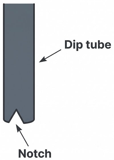
A way to help minimize this effect is to place small V-shaped notches at the end of the dip tube, to help bubbles escape at sizes smaller than the tube’s diameter:
Transmitter Suppression and Elevation
A very common scenario for liquid level measurement is where the pressure-sensing instrument is not located at the same level as the 0% measurement point. The following photograph shows an example of this, where a Rosemount model 3051 differential pressure transmitter is being used to sense hydrostatic pressure of colored water inside a (clear) vertical plastic tube:
Consider the example of a pressure sensor measuring the level of liquid ethanol in a storage tank. The measurement range for liquid height in this ethanol storage tank is 0 to 40 feet, but the transmitter is located 30 feet below the tank:
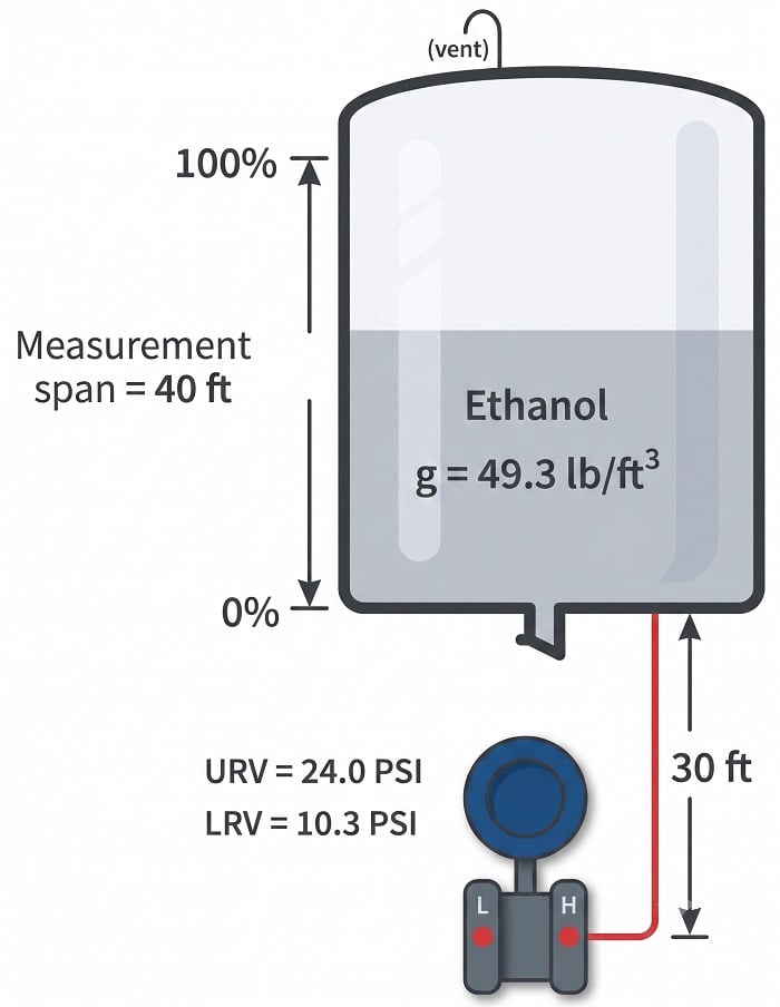
This means the transmitter’s impulse line contains a 30-foot elevation head of ethanol, so the transmitter “sees” 30 feet of ethanol when the tank is empty and 70 feet of ethanol when the tank is full. A 3-point calibration table for this instrument would look like this, assuming a 4 to 20 mA DC output signal range:
| Ethanol level | Percent of Range | Pressure ("W.C.) | Pressure (PSI) | Transmitter Output |
|---|---|---|---|---|
| 0 ft | 0 % | 284 "W.C. | 10.3 PSI | 4 mA |
| 20 ft | 50 % | 474 "W.C. | 17.1 PSI | 12 mA |
| 40 ft | 100 % | 663 "W.C. | 24.0 PSI | 20 mA |
Another common scenario is where the transmitter is mounted at or near the vessel’s bottom, but the desired level measurement range does not extend to the vessel bottom:
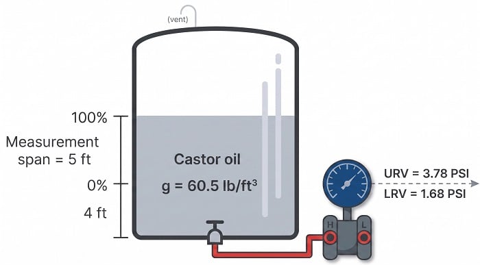
In this example, the transmitter is mounted exactly at the same level as the vessel bottom, but the level measurement range begins at 4 feet up from the vessel bottom. At the level of castor oil deemed 0%, the transmitter “sees” a hydrostatic pressure of 1.68 PSI (46.5 inches of water column) and at the 100% castor oil level the transmitter “sees” a pressure of 3.78 PSI (105 inches water column). Thus, these two pressure values would define the transmitter’s lower and upper range values (LRV and URV), respectively.
The term for describing either of the previous scenarios, where the lower range value (LRV) of the transmitter’s calibration is a positive number, is called zero suppression. If the zero offset is reversed (e.g. the transmitter mounted at a location higher than the 0% process level), it is referred to as zero elevation.
If the transmitter is elevated above the process connection point, it will most likely “see” a negative pressure (vacuum) with an empty vessel owing to the pull of liquid in the line leading down from the instrument to the vessel. It is vitally important in elevated transmitter installations to use a remote seal rather than an open impulse line, so liquid cannot dribble out of this line and into the vessel:
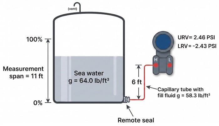
In this example, we see a remote seal system with a fill fluid having a density of 58.3 lb/ft\(^{3}\), and a process level measurement range of 0 to 11 feet of sea water (density = 64 lb/ft\(^{3}\)). The transmitter elevation is 6 feet, which means it will “see” a vacuum of \(-2.43\) PSI (\(-67.2\) inches of water column) when the vessel is completely empty. This, of course, will be the transmitter’s calibrated lower range value (LRV). The upper range value (URV) will be the pressure “seen” with 11 feet of sea water in the vessel. This much sea water will contribute an additional 4.89 PSI of hydrostatic pressure at the level of the remote seal diaphragm, causing the transmitter to experience a pressure of +2.46 PSI.
Compensated Leg Systems
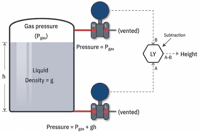
The simple and direct relationship between liquid height in a vessel and pressure at the bottom of that vessel is ruined if another source of pressure exists inside the vessel other than hydrostatic (elevation head). This is virtually guaranteed to be the case if the vessel in question is unvented. Any gas or vapor pressure accumulation in an enclosed vessel will add to the hydrostatic pressure at the bottom, causing any pressure-sensing instrument to falsely register a high level:
A pressure transmitter has no way of “knowing” how much of the sensed pressure is due to liquid elevation and how much of it is due to pressure existing in the vapor space above the liquid. Unless a way can be found to compensate for any non-hydrostatic pressure in the vessel, this extra pressure will be interpreted by the transmitter as additional liquid level.
Moreover, this error will change as gas pressure inside the vessel changes, so it cannot simply be “calibrated away” by a static zero shift within the instrument. The only way to hydrostatically measure liquid level inside an enclosed (non-vented) vessel is to continuously compensate for gas pressure.
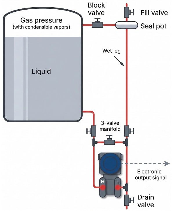
Fortunately, the capabilities of a differential pressure transmitter make this a simple task. All we need to do is connect a second impulse line (called a compensating leg), from the “Low” port of the transmitter to the top of the vessel, so the “Low” side of the transmitter experiences nothing but the gas pressure enclosed by the vessel, while the “High” side experiences the sum of gas and hydrostatic pressures. Since a differential pressure transmitter responds only to differences in pressure between “High” and “Low” sides, it will naturally subtract the gas pressure (\(P_{gas}\)) to yield a measurement based solely on hydrostatic pressure (\(\gamma h\)):
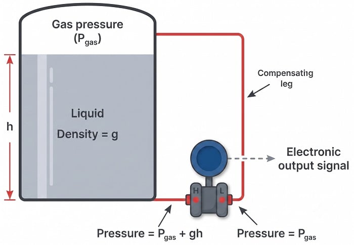
\[(P_{gas} + \gamma h) - P_{gas} = \gamma h\]
The amount of gas pressure inside the vessel now becomes completely irrelevant to the transmitter’s indication, because its effect is canceled at the differential pressure instrument’s sensing element. If gas pressure inside the vessel were to increase while liquid level remained constant, the pressure sensed at both ports of the differential pressure transmitter would increase by the exact same amount, with the pressure difference between the “high” and “low” ports remaining absolutely constant with the constant liquid level. This means the instrument’s output signal is a representation of hydrostatic pressure only, which represents liquid height (assuming a known liquid density \(\gamma\)).
Unfortunately, it is common for enclosed vessels to hold condensible vapors, which may over time fill a compensating leg full of liquid. If the tube connecting the “Low” side of a differential pressure transmitter fills completely with a liquid, this will add a hydrostatic pressure to that side of the transmitter, causing another calibration shift. This wet leg condition makes level measurement more complicated than a dry leg condition where the only pressure sensed by the transmitter’s “Low” side is gas pressure (\(P_{gas}\)):
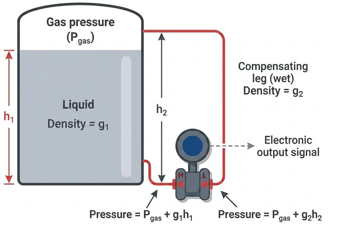
\[(P_{gas} + \gamma_1 h_1) - (P_{gas} + \gamma_2 h_2) = \gamma_1 h_1 - \gamma_2 h_2\]
Gas pressure still cancels due to the differential nature of the pressure transmitter, but now the transmitter’s output indicates a difference of hydrostatic pressures between the vessel and the wet leg, rather than just the hydrostatic pressure of the vessel’s liquid level. Fortunately, the hydrostatic pressure generated by the wet leg will be constant, so long as the density of the condensed vapors filling that leg (\(\gamma_2\)) is constant. If the wet leg’s hydrostatic pressure is constant, we can compensate for it by calibrating the transmitter with an intentional zero shift, so it indicates as though it were measuring hydrostatic pressure on a vented vessel.
\[\hbox{Differential pressure} = \gamma_1 h_1 - \hbox{Constant}\]
We may ensure a constant density of wet leg liquid by intentionally filling that leg with a liquid known to be denser than the densest condensed vapor inside the vessel and non-miscible with the process fluid. We could also use a differential pressure transmitter with remote seals and capillary tubes filled with liquid of known density:
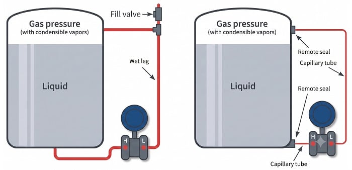
Remote seals are very useful in applications such as this, as the wet leg never requires re-filling.
An actual level transmitter installation using two remote seals (in this case, a Foxboro IDP10 differential pressure transmitter) appears in this photograph:
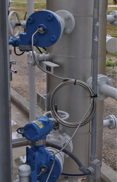
The vessel itself is insulated, and covered in sheet aluminum to protect the thermal insulation from impact and weather-related damage. White-painted flanged “nozzles” protrude from the vessel through the insulation to provide places for the level-sensing instrument to connect. You can see the two flanged remote seals (painted blue) where the armored (stainless steel) capillary tubes terminate. Note how the long capillary tube on the “wet” leg is neatly coiled to reduce the possibility of damage by snagging on any moving object.
An accessory commonly used with non-sealed (non-capillary) “wet leg” systems is a seal pot. This is a chamber at the top of the wet leg joining the wet leg line with the impulse line to the upper connection point on the process vessel. This “seal pot” maintains a small volume of liquid in it to allow for occasional liquid loss during transmitter maintenance procedures without greatly affecting the height of the liquid column in the wet leg:
Regular operation of the transmitter’s three-valve manifold (and drain valve) during routine instrument maintenance inevitably releases some liquid volume from the wet leg. Without a seal pot, even a small loss of liquid in the wet leg may create a substantial loss in liquid column height within that tube, given the tube’s small diameter. With a seal pot, the (comparatively) large liquid volume held by the pot allows for some liquid loss through the transmitter’s manifold without substantially affecting the height of the liquid column within the wet leg.
Seal pots are standard on level measurement systems for boiler steam drums, where steam readily condenses in the upper impulse tube to naturally form a wet leg. Although steam will condense over time to refill the wet leg following a loss of water in that leg, the level measurements taken during that re-fill time will be in error. The presence of a seal pot practically eliminates this error as the steam condenses to replenish the water lost from the pot, since the amount of height change inside the pot due to a small volume loss is trivial compared to the height change in a wet leg lacking a seal pot.
The following example shows the calibration table for a compensated-leg (wet) hydrostatic level measurement system, for a gasoline storage vessel and water as the wet leg fill fluid. Here, I am assuming a density of 41.0 lb/ft\(^{3}\) for gasoline and 62.4 lb/ft\(^{3}\) for water, with a 0 to 10 foot measurement range and an 11 foot wet leg height:
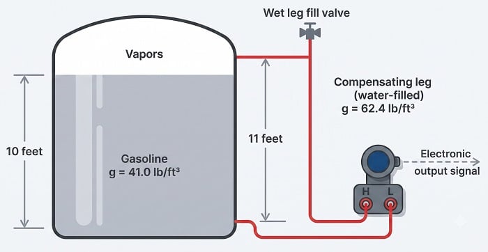
| Gasoline level | Percent of Range | Differential Pressure | Transmitter Output |
|---|---|---|---|
| 0 ft | 0 % | -4.77 PSI | 4 mA |
| 2.5 ft | 25 % | -4.05 PSI | 8 mA |
| 5 ft | 50 % | -3.34 PSI | 12 mA |
| 7.5 ft | 75 % | -2.63 PSI | 16 mA |
| 10 ft | 100 % | -1.92 PSI | 20 mA |
Note that due to the superior density and height of the wet (water) leg, the transmitter always sees a negative pressure (pressure on the “Low” side exceeds pressure on the “High” side).
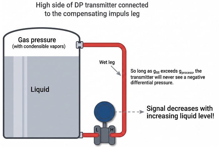
With some older differential pressure transmitter designs, this negative pressure was a problem. Consequently, it is common to see “wet leg” hydrostatic transmitters installed with the “Low” port connected to the bottom of the vessel and the “High” port connected to the compensating leg. In fact, it is still common to see modern differential pressure transmitters installed in this manner, although modern transmitters may be ranged for negative pressures just as easily as for positive pressures. It is vitally important to recognize that any differential pressure transmitter connected as such (for any reason) will respond in reverse fashion to increases in liquid level. That is to say, as the liquid level in the vessel rises, the transmitter’s output signal will decrease instead of increase:
Either way of connecting the transmitter to the vessel will suffice for measuring liquid level, so long as the instrumentation receiving the transmitter’s signal is properly configured to interpret the signal. The choice of which way to connect the transmitter to the vessel should be driven by fail-safe system design, which means to design the measurement system such that the most probable system failures – including broken signal wires – result in the control system “seeing” the most dangerous process condition and therefore taking the safest action.
Tank Expert Systems
An alternative to using a compensating leg to subtract gas pressure inside an enclosed vessel is to simply use a second pressure transmitter and electronically subtract the two pressures in a computing device:
This approach enjoys the distinct advantage of avoiding a potentially wet compensating leg, but suffers the disadvantages of extra cost and greater error due to the potential calibration drift of two transmitters rather than just one. Such a system is also impractical in applications where the gas pressure is substantial compared to the hydrostatic (elevation head) pressure.
If we add a third pressure transmitter to this system, located a known distance (\(x\)) above the bottom transmitter, we have all the pieces necessary for what is called a tank expert system. These systems are used on large storage tanks operating at or near atmospheric pressure, and have the ability to measure infer liquid height, liquid density, total liquid volume, and total liquid mass stored in the tank:
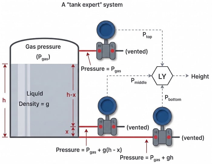
The pressure difference between the bottom and middle transmitters will change only if the liquid density changes, since the two transmitters are separated by a known and fixed height difference.
Algebraic manipulation shows us how the measured pressures may be used by the level computer (LY) to continuously calculate liquid density (\(\gamma\)):
\[P_{bottom} - P_{middle} = (P_{gas} + \gamma h) - [P_{gas} + \gamma (h - x)]\]
\[P_{bottom} - P_{middle} = P_{gas} + \gamma h - P_{gas} - \gamma (h - x)\]
\[P_{bottom} - P_{middle} = P_{gas} + \gamma h - P_{gas} - \gamma h + \gamma x\]
\[P_{bottom} - P_{middle} = \gamma x\]
\[{{P_{bottom} - P_{middle}} \over x} = \gamma\]
Once the computer knows the value of \(\gamma\), it may calculate the height of liquid in the tank with great accuracy based on the pressure measurements taken by the bottom and top transmitters:
\[P_{bottom} - P_{top} = (P_{gas} + \gamma h) - P_{gas}\]
\[P_{bottom} - P_{top} = \gamma h\]
\[{{P_{bottom} - P_{top}} \over \gamma} = h\]
With all the computing power available in the LY, it is possible to characterize the tank such that this height measurement converts to a precise volume measurement (\(V\)), which may then be converted into a total mass (\(m\)) measurement based on the mass density of the liquid (\(\rho\)) and the acceleration of gravity (\(g\)). First, the computer calculates mass density based on the proportionality between mass and weight (shown here starting with the equivalence between the two forms of the hydrostatic pressure formula):
\[\rho g h = \gamma h\]
\[\rho g = \gamma\]
\[\rho = {\gamma \over g}\]
Armed with the mass density of the liquid inside the tank, the computer may now calculate total liquid mass stored inside the tank:
\[m = \rho V\]
Dimensional analysis shows how units of mass density and volume cancel to yield only units of mass in this last equation:
\[\left[\hbox{kg}\right] = \left[\hbox{kg} \over \hbox{m}^3\right] \left[\hbox{m}^3\right]\]
Here we see a vivid example of how several measurements may be inferred from just a few actual process (in this case, pressure) measurements. Three pressure measurements on this tank allow us to compute four inferred variables: liquid density, liquid height, liquid volume, and liquid mass.
The accurate measurement of liquids in storage tanks is not just useful for process operations, but also for conducting business. Whether the liquid represents raw material purchased from a supplier, or a processed product ready to be pumped out to a customer, both parties have a vested interest in knowing the exact quantity of liquid bought or sold. Measurement applications such as this are known as custody transfer, because they represent the transfer of custody (ownership) of a substance exchanged in a business agreement. In some instances, both buyer and seller operate and maintain their own custody transfer instrumentation, while in other instances there is only one instrument, the calibration of which validated by a neutral party.
A photograph showing the two lower pressure transmitters of a tank expert system on a refrigerated butane storage vessel appears here:
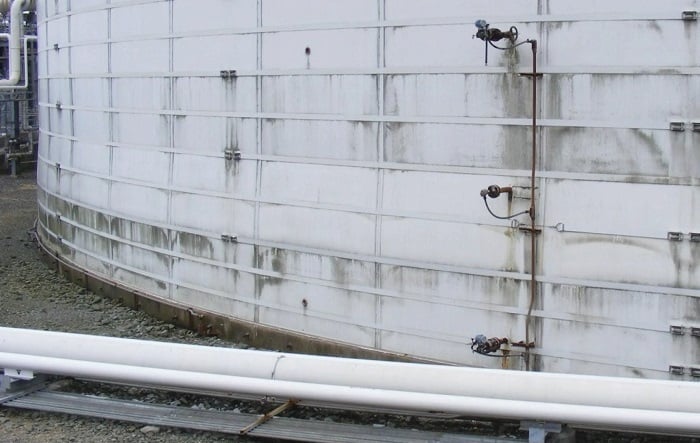
The upper and lower instruments are pressure transmitters, while the middle instrument is a temperature sensor used to report the temperature of the refrigerated butane to the control system.
Hydrostatic Interface Level Measurement
Hydrostatic pressure sensors may be used to detect the level of a liquid-liquid interface, if and only if the total height of liquid never drops down into the sensing range of the interface level instrument. This is critically important because any single hydrostatic-based level instrument cannot discriminate between a changing interface level and a changing total level within the same range, and therefore the latter must be fixed in order to measure the former.
One way to ensure this condition is to fix the total liquid height to some constant value by using an overflow pipe, and ensuring drain flow is always less than incoming flow (forcing some flow to always go through the overflow pipe). This strategy naturally lends itself to separation processes, where a mixture of light and heavy liquids are separated by their differing densities:
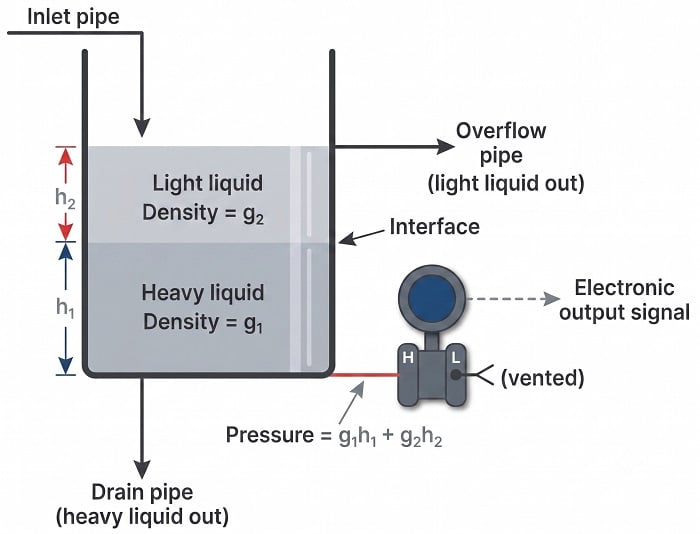
Here we see a practical application for liquid-liquid interface level measurement. If the goal is to separate two liquids of differing densities from one another, we need only the light liquid to exit out the overflow pipe and only the heavy liquid to exit out the drain pipe. This means we must control the interface level to stay between those two piping points on the vessel. If the interface drifts too far up, heavy liquid will be carried out the overflow pipe; and if we let the interface drift too far down, light liquid will flow out of the drain pipe. The first step in controlling any process variable is to measure that variable, and so here we are faced with the necessity of measuring the interface point between the light and heavy liquids.
Another way to address the problem of varying total liquid height is to use a compensating leg located at a point on the vessel below the total liquid height. In this example, a transmitter with remote seals is used:
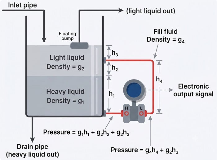
Since both sides of the differential pressure transmitter “see” the hydrostatic pressure generated by the liquid column above the top connection point (\(\gamma_2 h_3\)), this term naturally cancels. The result of this is that total liquid height becomes irrelevant, so long as it remains above the upper connection point:
\[(\gamma_1 h_1 + \gamma_2 h_2 + \gamma_2 h_3) - (\gamma_4 h_4 + \gamma_2 h_3)\]
\[\gamma_1 h_1 + \gamma_2 h_2 + \gamma_2 h_3 - \gamma_4 h_4 - \gamma_2 h_3\]
\[\gamma_1 h_1 + \gamma_2 h_2 - \gamma_4 h_4\]
The hydrostatic pressure in the compensating leg is constant (\(\gamma_4 h_4\) = Constant), since the fill fluid never changes density and the compensating leg’s height never changes. This means the transmitter’s sensed pressure will differ from that of an uncompensated transmitter merely by a constant offset, which may be “calibrated out” so as to have no impact on the measurement:
\[\gamma_1 h_1 + \gamma_2 h_2 - \hbox{Constant}\]
At first, it may seem as though determining the calibration points (lower- and upper-range values: LRV and URV) for a hydrostatic interface level transmitter is impossibly daunting given all the different pressures involved. A recommended problem-solving technique to apply here is that of a thought experiment, where we imagine what the process will “look like” at lower-range value condition and at the upper-range value condition, drawing two separate illustrations:
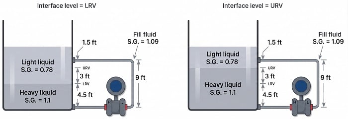
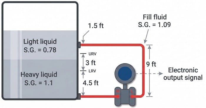
For example, suppose we must calibrate a differential pressure transmitter to measure the interface level between two liquids having specific gravities of 1.1 and 0.78, respectively, over a span of 3 feet. The transmitter is equipped with remote seals, each containing a halocarbon fill fluid with a specific gravity of 1.09. The physical layout of the system is as follows:
As the first step in our “thought experiment,” we imagine what the process would look like with the interface at the LRV level, calculating hydrostatic pressures seen at each side of the transmitter. For this I recommend actually sketching a simple diagram showing what the fluid levels would look like with the interface at the LRV point, so the height dimensions of each liquid layer become obvious:
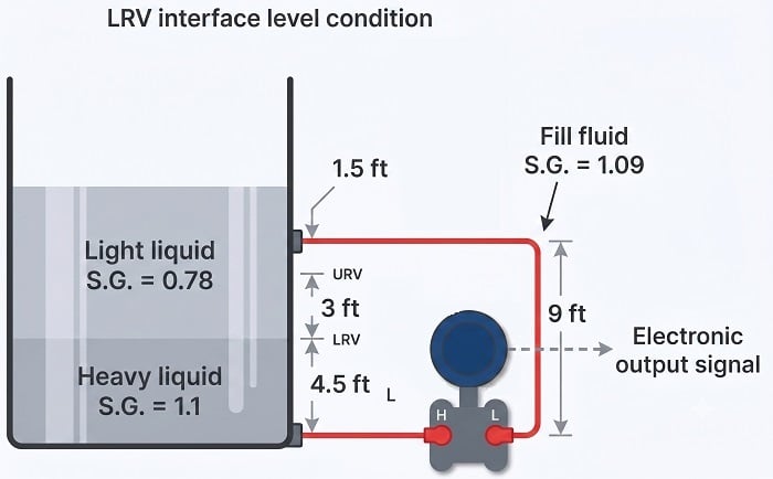
We know from our previous exploration of this setup that any hydrostatic pressure resulting from liquid level above the top remote seal location is irrelevant to the transmitter, since it is “seen” on both sides of the transmitter and thus cancels out. All we must do, then, is calculate hydrostatic pressures as though the total liquid level stopped at that upper diaphragm connection point.
First, calculating the hydrostatic pressure “seen” at the high port of the transmitter:
\[P_{high} = 4.5 \hbox{ feet of heavy liquid} + 4.5 \hbox{ feet of light liquid}\]
\[P_{high} = 54 \hbox{ inches of heavy liquid} + 54 \hbox{ inches of light liquid}\]
\[P_{high} \hbox{ "W.C.} = (54 \hbox{ inches of heavy liquid})(1.1) + (54 \hbox{ inches of light liquid})(0.78)\]
\[P_{high} \hbox{ "W.C.} = 59.4 \hbox{ "W.C.} + 42.12 \hbox{ "W.C.}\]
\[P_{high} = 101.52 \hbox{ "W.C.}\]
Next, calculating the hydrostatic pressure “seen” at the low port of the transmitter:
\[P_{low} = 9 \hbox{ feet of fill fluid}\]
\[P_{low} = 108 \hbox{ inches of fill fluid}\]
\[P_{low} \hbox{ "W.C.} = (108 \hbox{ inches of fill fluid})(1.09)\]
\[P_{low} = 117.72 \hbox{ "W.C.}\]
The differential pressure applied to the transmitter in this condition is the difference between the high and low port pressures, which becomes the lower range value (LRV) for calibration:
\[P_{LRV} = 101.52 \hbox{ "W.C.} - 117.72 \hbox{ "W.C.} = -16.2 \hbox{ "W.C.}\]
As the second step in our “thought experiment,” we imagine what the process would look like with the interface at the URV level, calculating hydrostatic pressures seen at each side of the transmitter. Again, sketching a simple diagram of what the liquid layers would look like in this condition helps us visualize the scenario:
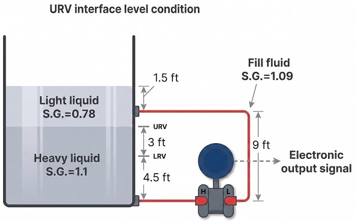
\[P_{high} = 7.5 \hbox{ feet of heavy liquid} + 1.5 \hbox{ feet of light liquid}\]
\[P_{high} = 90 \hbox{ inches of heavy liquid} + 18 \hbox{ inches of light liquid}\]
\[P_{high} \hbox{ "W.C.} = (90 \hbox{ inches of heavy liquid})(1.1) + (18 \hbox{ inches of light liquid})(0.78)\]
\[P_{high} \hbox{ "W.C.} = 99 \hbox{ "W.C.} + 14.04 \hbox{ "W.C.}\]
\[P_{high} = 113.04 \hbox{ "W.C.}\]
The hydrostatic pressure of the compensating leg is exactly the same as it was before: 9 feet of fill fluid having a specific gravity of 1.09, which means there is no need to calculate it again. It will still be 117.72 inches of water column. Thus, the differential pressure at the URV point is:
\[P_{URV} = 113.04 \hbox{ "W.C.} - 117.72 \hbox{ "W.C.} = -4.68 \hbox{ "W.C.}\]
Using these two pressure values and some interpolation, we may generate a 5-point calibration table (assuming a 4-20 mA transmitter output signal range) for this interface level measurement system:
| Interface level | Percent of Range | Differential Pressure | Transmitter Output |
|---|---|---|---|
| 4.5 ft | 0 % | -16.2 "W.C. | 4 mA |
| 5.25 ft | 25 % | -13.32 "W.C. | 8 mA |
| 6 ft | 50 % | -10.44 "W.C. | 12 mA |
| 6.75 ft | 75 % | -7.56 "W.C. | 16 mA |
| 7.5 ft | 100 % | -4.68 "W.C. | 20 mA |
When the time comes to bench-calibrate this instrument in the shop, the easiest way to do so will be to set the two remote diaphragms on the workbench (at the same level), then apply 16.2 to 4.68 inches of water column pressure to the low remote seal diaphragm with the other diaphragm at atmospheric pressure to simulate the desired range of negative differential pressures.
The more mathematically inclined reader will notice that the span of this instrument (Span = URV \(-\) LRV) is equal to the span of the interface level (3 feet, or 36 inches) multiplied by the difference in specific gravities (1.1 \(-\) 0.78):
\[\hbox{Span in "W.C.} = (36 \hbox{ inches})(1.1 - 0.78)\]
\[\hbox{Span} = 11.52 \hbox{ "W.C.}\]
Looking at our two “thought experiment” illustrations, we see that the only difference between the two scenarios is the type of liquid filling that 3-foot region between the LRV and URV marks. Therefore, the only difference between the transmitter’s pressures in those two conditions will be the difference in height multiplied by the difference in density. Not only is this an easy way for us to quickly calculate the necessary transmitter span, but it also is a way for us to check our previous work: we see that the difference between the LRV and URV pressures is indeed a difference of 11.52 inches water column just as this method predicts.
