 Facebook
 Google
 GitHub
 Linkedin
FOUNDATION Fieldbus H1 Protocol Device Configuration and Commissioning
Fieldbus devices require far more attention in their initial setup and commissioning than their analog counterparts. Unlike an analog transmitter, for example, where the only “configuration” settings are its zero and span calibration adjustments, a FF transmitter has a substantial number of parameters describing its behavior. Some of these parameters must be set by the end-user, while others are configured automatically by the host system during the start-up process, which we generally refer to as commissioning.
Configuration files
In order for a FF device to work together with a host system (which may be manufactured by a different company), the device must have its capabilities explicitly described so the host system “knows what to do with it.” This is analogous to the need for driver files when interfacing a personal computer with a new peripheral device such as a printer, scanner, or modem.
A standardized language exists for digital instrumentation called the Device Description Language, or DDL. All FF instrument manufacturers are required to document their devices’ capabilities in this standard-format language, which is then compiled by a computer into a set of files known as the Device Description (DD) files for that instrument. DDL itself is a text-based language, much like C or Java, written by a human programmer. The DD files are generated from the DDL source file by a computer, output in a form intended for another computer’s read-only access. For FF instruments, the DD files end in the filename extensions .sym and .ffo, and may be obtained freely from the manufacturer or from the Fieldbus Foundation website (http://www.fieldbus.org). The .ffo DD file is in a binary format readable only by a computer with the appropriate “DD services” software active. The .sym DD file is ASCII-encoded, making it viewable by a human by using a text editor program (although you should not attempt to edit the contents of a .sym file).
Other device-specific files maintained by the host system of a FF segment are the Capability and Value files, both referred to as Common Format Files, or .cff files. These are also text-readable (ASCII encoded) digital files describing device capability and specific configuration values for the device, respectively. The Capability file for a FF device is typically downloaded from either the manufacturer’s or the Fieldbus Foundation website along with the two DD files, as a three-file set (filename extensions being .cff, .sym, and .ffo, respectively). The Value file is generated by the host system during the device’s configuration, storing the specific configuration values for that specific device and system tag number. The data stored in a Value file may be used to duplicate the exact configuration of a failed FF device, ensuring the new device replacing it will contain all the same parameters.
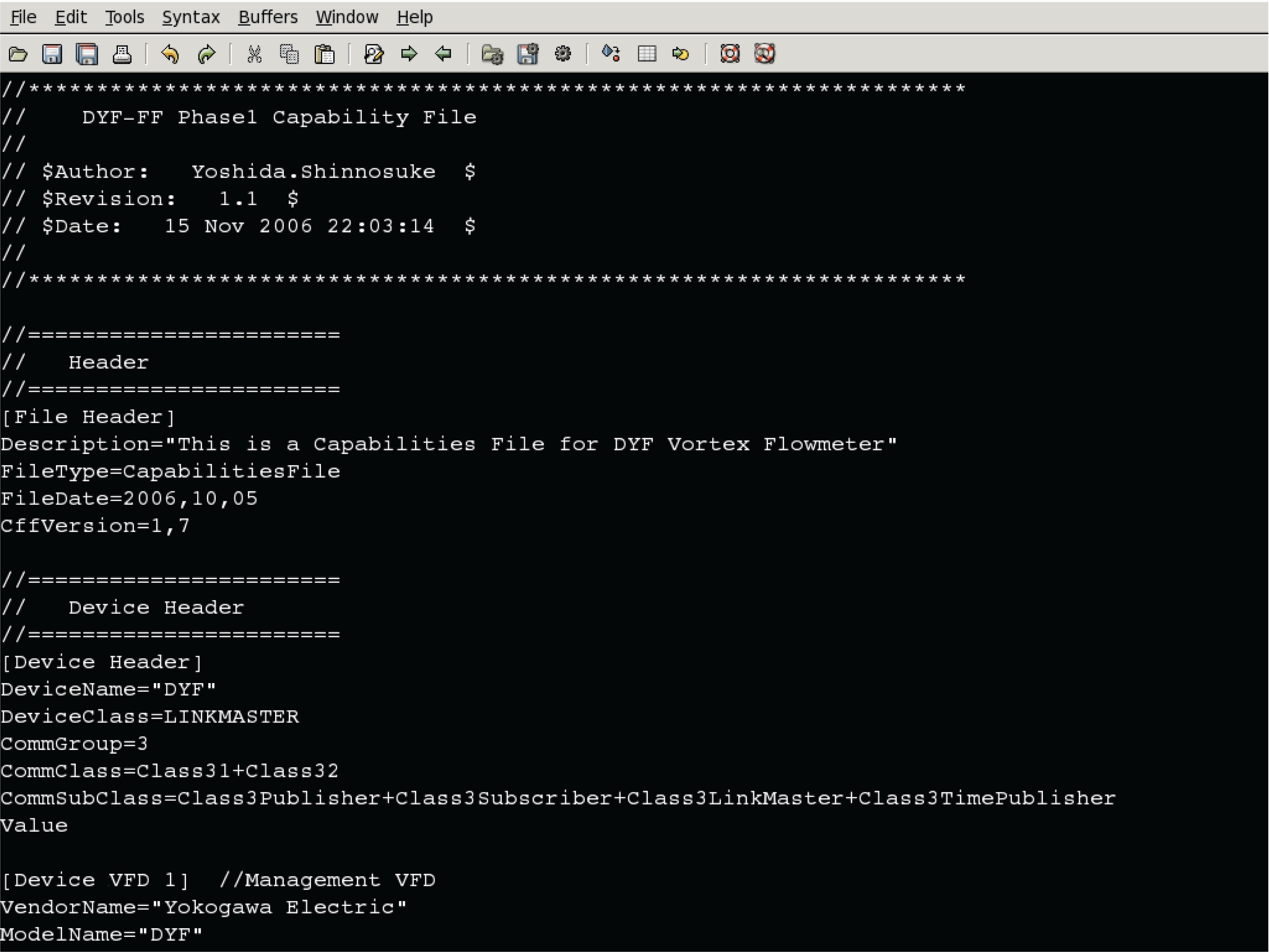
A screenshot of a .cff Capability file opened in a text editor program appears here, showing the first few lines of code describing the capabilities of a Yokogawa model DYF vortex flowmeter:
As with “driver” files needed to make a personal computer peripheral device function, it is important to have the correct versions of the Capability and DD files installed on the host system computer before attempting to commission the device. It is permissible to have Capability and DD files installed that are newer than the physical device, but not vice-versa (a newer physical device than the Capability and DD files). This requirement of proper configuration file management is a new task for the instrument technician and engineer to manage in their jobs. With every new FF device installed in a control system, the proper configuration files must be obtained, installed, and archived for safe keeping in the event of data loss (a “crash”) in the host system.
Device commissioning
This section illustrates the commissioning of a Fieldbus device on a real segment, showing screenshots of a host system’s configuration menus. The particular device happens to be a Fisher DVC5000f valve positioner, and the host system is a DeltaV distributed control system manufactured by Emerson. All configuration files were updated in this system prior to the commissioning exercise. Keep in mind that the particular steps taken to commission any FF device will vary from one host system to another, and may not follow the sequence of steps shown here.
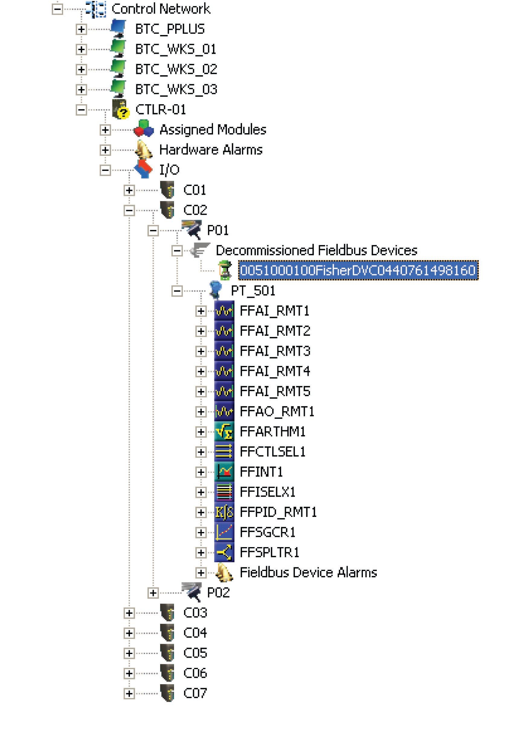
If an unconfigured FF device is connected to an H1 network, it appears as a “decommissioned” device. On the Emerson DeltaV host system, all decommissioned FF devices appear within a designated folder on the “container” hierarchy. Here, my Fisher DVC5000 device is shown highlighted in blue. A commissioned FF device appears just below it (PT_501), showing all available function blocks within that instrument:
Before any FF device may be recognized by the DeltaV host system, a “placeholder” and tag name must be created for it within the segment hierarchy. To do this, a “New Fieldbus Device” must be added to the H1 port. Once this option is selected, a window opens up to allow naming of this new device:
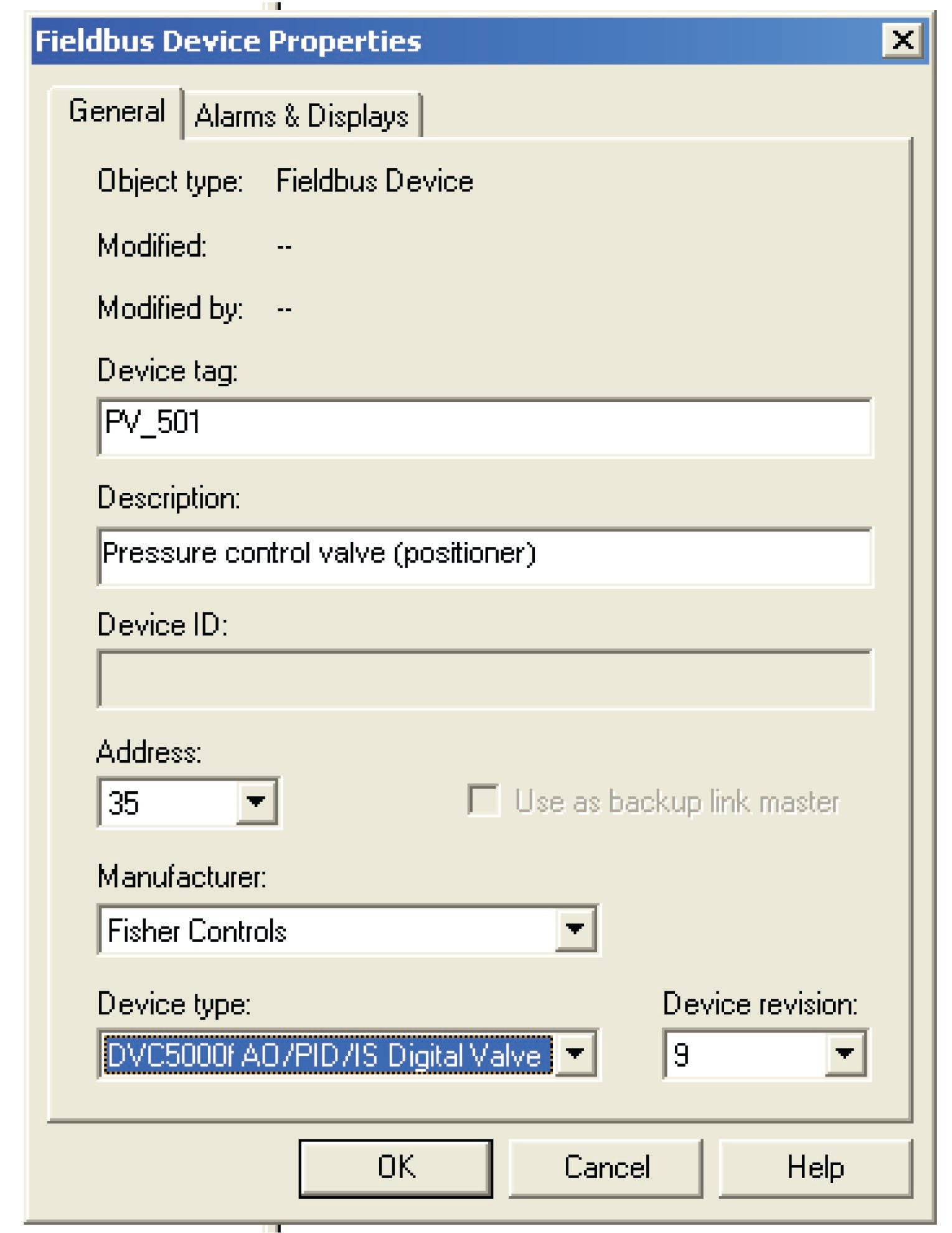
Here, the tag name “PV_501” has been chosen for the Fisher valve positioner, since it will work in conjunction with the pressure transmitter PT_501 to form a complete pressure control loop. In addition to a tag name (PV_501), I have also added a text description (“Pressure control valve (positioner)”), and specified the device type (Fisher DVC5000f with AO, PID, and IS function block capability). The DeltaV host system chose a free address for this device (35), although it is possible to manually select the desired device address at this point. Note the “Backup Link Master” check box in this configuration window, which is grey in color (indicating the option is not available with this device).
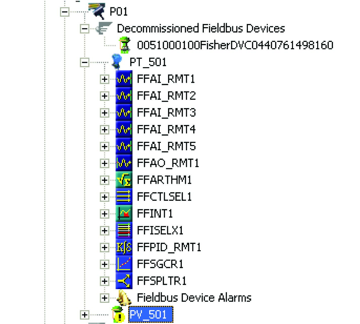
After the device information has been entered for the new tag name, a “placeholder” icon appears within the hierarchy for the H1 segment (connected to Port 1). You can see the new tag name (PV_501) below the last function block for the commissioned FF instrument (PT_501). The actual device is still decommissioned, and appears as such:
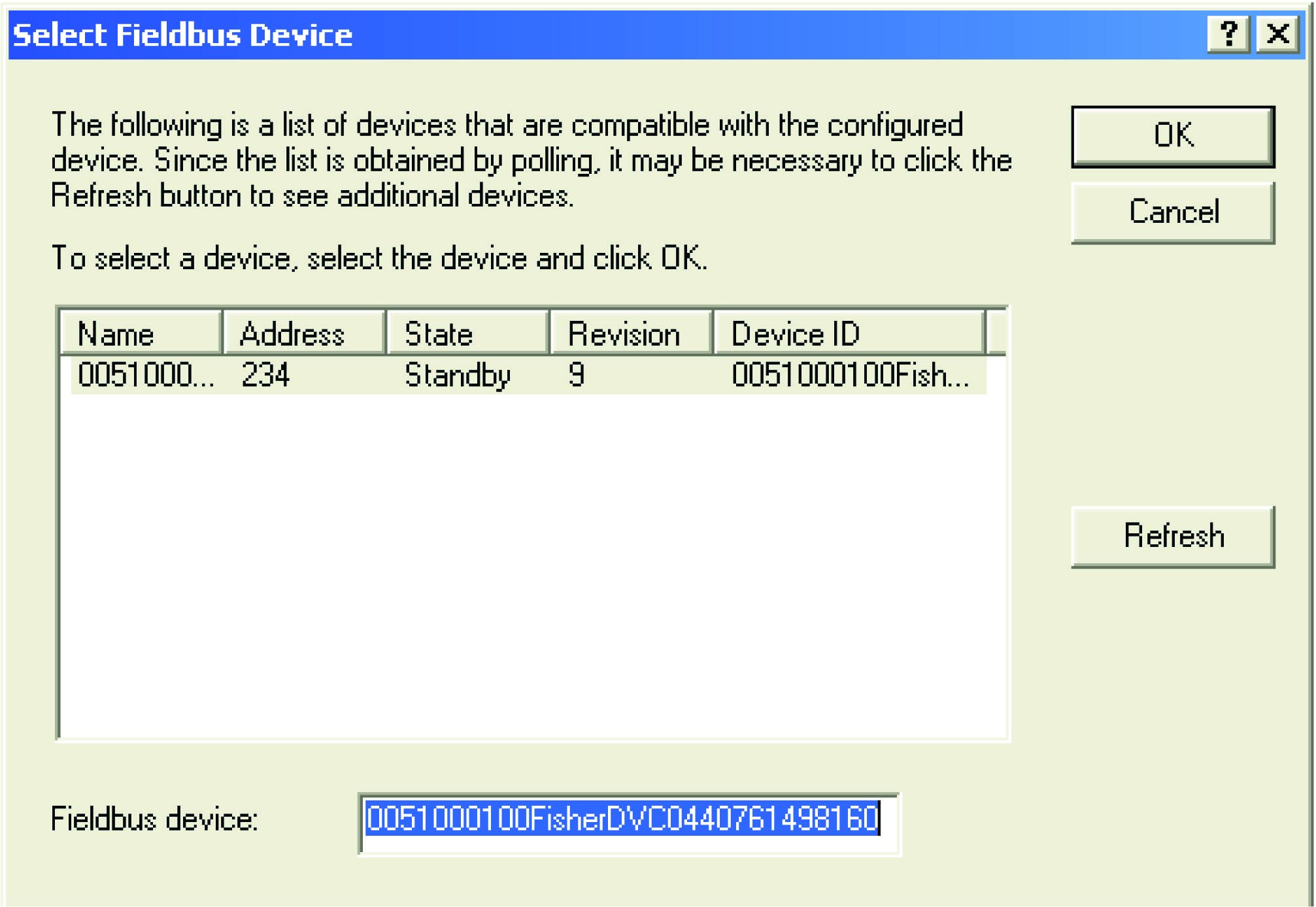
By right-clicking on the new tag name and selecting the “Commission” option, a new window opens to allow you to select which decommissioned device should be given the new tag name. Since there is only one decommissioned device on this particular H1 segment, only one option appears within the window:
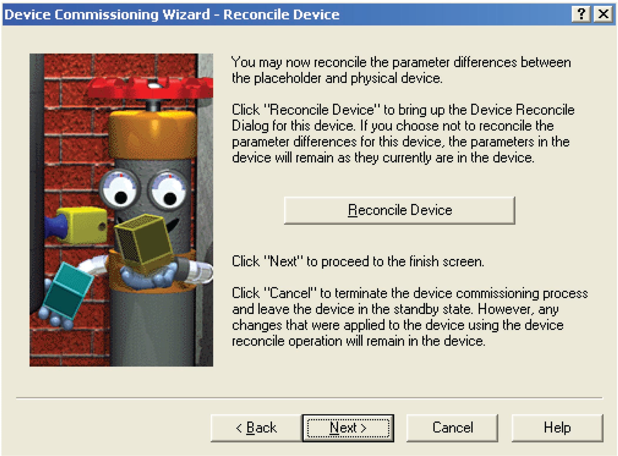
After selecting the decommissioned device you wish to commission, the DeltaV host system prompts you to reconcile any differences between the newly created tag name placeholder and the decommissioned device. If you want to use the existing values stored within the physical (decommissioned) device, you skip the “reconcile” step. If you want to alter the values in the device from what they presently are, you choose the “reconcile” option which then opens up an editing window where you can set the device values however you wish.
After selecting (or not selecting) the “reconcile” option, the DeltaV system prompts you to confirm commissioning of the device, after which it goes through a series of animated display sequences as the device transitions from the “Standby” state to the “Commissioned” state:
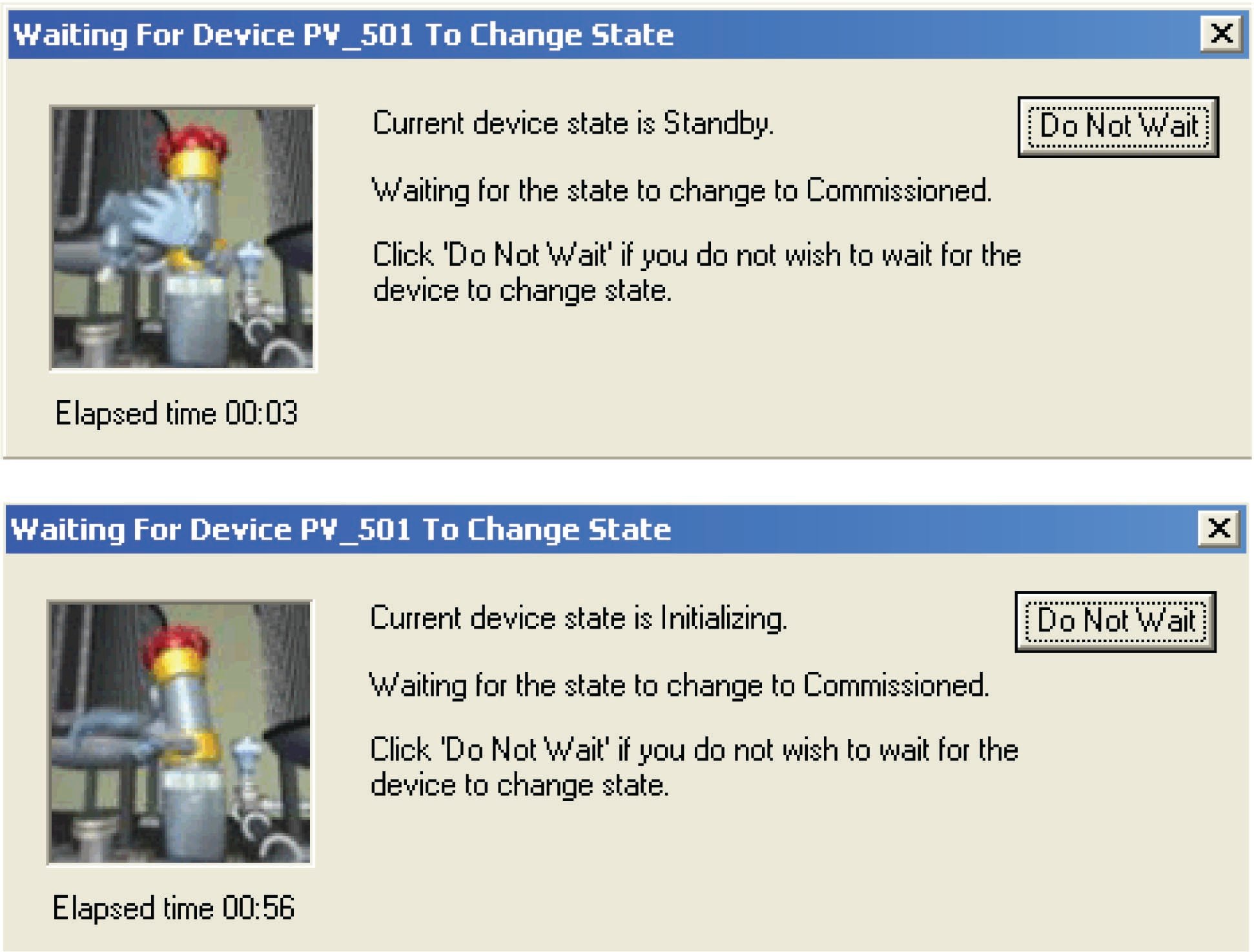
As you can see, the commissioning process is not very fast. After nearly one full minute of waiting, the device is still “Initializing” and not yet “Commissioned.” The network speed of 31.25 kbps and the priority of scheduled communications are limiting factors when exchanging large quantities of configuration data over a FF H1 network segment. In order for device configuration to not interrupt or slow down process-critical data transfers, all configuration data exchanges must wait for unscheduled time periods, and then transmit at the relatively slow rate of 31.25 kbps when the alloted times arrive. Any technician accustomed to the fast data transfer rates of modern Ethernet devices will feel as though he or she has taken a step back in time when computers were much slower.
After commissioning this device on the DeltaV host system, several placeholders in the hierarchy appear with blue triangles next to them. In the DeltaV system, these blue triangle icons represent the need to download database changes to the distributed nodes of the system:

After “downloading” the data, the new FF valve positioner shows up directly below the existing pressure transmitter as a commissioned instrument, and is ready for service. The function blocks for pressure transmitter PT_501 have been “collapsed” back into the transmitter’s icon, and the function blocks for the new valve positioner (PV_501) have been “expanded” for view:

As you can see, the new instrument (PV_501) does not offer nearly as many function blocks as the original FF instrument (PT_501). The number of Fieldbus function blocks offered by any FF instrument is a function of that instrument’s computational ability, internal task loading, and the discretion of its designers. Obviously, this is an important factor to consider when designing a FF segment: being sure to include instruments that contain all the necessary function blocks to execute the desired control scheme. This may also become an issue if one of the FF instruments in a control scheme is replaced with one of a different manufacturer or model, having fewer available function blocks. If one or more mission-critical function blocks is not available in the replacement instrument, a different replacement must be sought.
Calibration and ranging
Calibration and ranging for a FF device is similar in principle to any other “smart” measurement instrument. Unlike analog instruments, where the “zero” and “span” adjustments completely define the instrument’s calibration and range, calibration and ranging are two completely different functions in a digital instrument.
To begin, we will examine a block diagram of an analog pressure transmitter showing the zero and span adjustments, with analog signaling between all functions inside the transmitter:

The “zero” and “span” adjustments together define the mathematical relationship between sensed pressure and current output. Calibration of an analog transmitter consists of applying known (reference standard) input stimuli to the instrument, and adjusting the “zero” and “span” settings until the desired current output values are achieved. The goal in doing this is to ensure accuracy of measurement.
The “range” of a transmitter is simply the input values associated with 0% and 100% output signals (e.g. 4 mA and 20 mA). Ranging an analog transmitter consists (also) of adjusting the “zero” and “span” settings until the output signal corresponds to the desired LRV and URV points of the measured variable. For an analog transmitter, the functions of ranging and calibration are always performed by the technician at the same time: to calibrate an analog transmitter is to range it, and vice-versa.
By contrast, a “smart” (digital) transmitter equipped with an analog 4-20 mA current output distinctly separates the calibration and range functions, each function determined by a different set of adjustments:

Calibration of a “smart” transmitter consists of applying known (reference standard) input stimuli to the instrument and engaging the “trim” functions until the instrument accurately registers the input stimuli. For a “smart” transmitter equipped with analog electronic (4-20 mA) output, there are two sets of calibration trim adjustments: one for the analog-to-digital converter and another for the digital-to-analog converter.
Ranging, by contrast, establishes the mathematical relationship between the measured input value and the output current value. To illustrate the difference between calibration and ranging, consider a case where a pressure transmitter is used to measure water pressure in a pipe. Suppose the transmitter’s pressure range of 0 to 100 PSI translates to a 4-20 mA output current. If we desired to re-range an analog transmitter to measure a greater span of pressures (say, 0 to 150 PSI), we would have to re-apply known pressures of 0 PSI and 150 PSI while adjusting the zero and span potentiometers so 0 PSI input gave a 4 mA output value and 150 PSI input gave a 20 mA output value. The only way to re-range an analog transmitter is to completely re-calibrate it.
In a “smart” (digital) measuring instrument, however, calibration against a known (standard) source need only be done at the specified intervals to ensure accuracy over long periods of time given the instrument’s inevitable drift. If our hypothetical transmitter were recently calibrated against a known pressure standard and trusted not to have drifted since the last calibration cycle, we could re-range it by simply changing the URV (upper range value) so that an applied pressure of 150 PSI now commands it to output 20 mA instead of an applied pressure of 100 PSI as was required before. Digital instrumentation allows us to re-range without re-calibrating, representing a tremendous savings in technician time and effort.
The distinction between calibration and ranging tends to confuse people, even some experienced technicians. When working with an analog transmitter, you cannot calibrate without setting the instrument’s range as well: the two functions are merged in the same procedures of adjusting zero and span. When working with a digital transmitter, however, the function of calibration and the function of ranging are entirely separate.
For a detailed analogy explaining the distinction between calibration and ranging, refer to section 18.6 beginning on page .
Fieldbus instruments, of course, are “smart” in the same way, and their internal block diagrams look much the same as the “smart” transmitters with analog current output, albeit with a far greater number of parameters within each block. The rectangle labeled “XD” in the following diagram is the Transducer block, while the rectangle labeled “AI” is the Analog Input block:

Calibration (trim) values are set in the transducer block along with the engineering unit, making the output of the transducer block a digital value scaled in real units of measurement (e.g. PSI, kPa, bar, mm Hg, etc.) rather than an abstract ADC “count” value. The analog input function block’s Channel parameter tells it which transducer output to receive as the pre-scaled “Primary Value”, which it may then translate to another scaled value based on a proportionality between transducer scale values (XD_Scale high and low) and output scale values (OUT_Scale high and low).
To calibrate such a transmitter, the transducer block should first be placed in Out Of Service (OOS) mode using a handheld FF communicator or the Fieldbus host system. Next, a standard (calibration-grade) fluid pressure is applied to the transmitter’s sensor and the Cal_Point_Lo parameter is set to equal this applied pressure. After that, a greater pressure is applied to the sensor and the Cal_Point_Hi parameter is set to equal this applied pressure. After setting the various calibration record-keeping parameters (e.g. Sensor_Cal_Date, Sensor_Cal_Who), the transducer block’s mode may be returned to Auto and the transmitter used once again.
To range such a transmitter, a correspondence between sensed pressure and the process variable must be determined and entered into the analog input function block’s XD_Scale and OUT_Scale parameters. If the pressure transmitter is being used to indirectly measure something other than pressure, these range parameters will become very useful, not only proportioning the numerical values of the measurement, but also casting the final digital output value into the desired “engineering units” (units of measurement).
Ranging in Fieldbus transmitters is a somewhat confusing topic due to the unfortunate names given to the different L_Type parameter options. Here is a list of the L_Type parameter options along with their meanings:
- = the AI block will publish the signal output by the XD block, regardless of the specified
OUT_Scalerange - = the AI block will mathematically scale the signal from the XD block into a range specified by
OUT_Scaleparameters using a linear equation (e.g. \(y = mx + b\)) - = same as above, except that a square-root function is applied to the percentage of range (useful when characterizing flow transmitters based on differential pressure measurement)
The terms “direct” and “indirect” are unfortunate, because they often cause people to interpret them as “direct” and “reverse” (as though L_Type described the direction of action for the function block). This is not what these terms mean for the AI block! What a “direct” value for L_Type means is that the raw value of the XD block is what will be published onto the Fieldbus network by the AI block. What an “indirect” value for L_Type means is that the XD block’s signal will be scaled to a different range (specified by the OUT_Scale parameter). In summary, the technician must set the XD_Scale range according to the primary signal sensed by the transmitter’s sensing element, and set the OUT_Scale range according to what the rest of the control system needs to see proportional to that primary signal.
The concept of ranging a FF transmitter makes more sense when viewed in the context of a real application. Consider this example, where a pressure transmitter is being used to measure the level of ethanol (ethyl alcohol) stored in a 40 foot high tank. The transmitter connects to the bottom of the tank by a tube, and is situated 10 feet below the tank bottom:
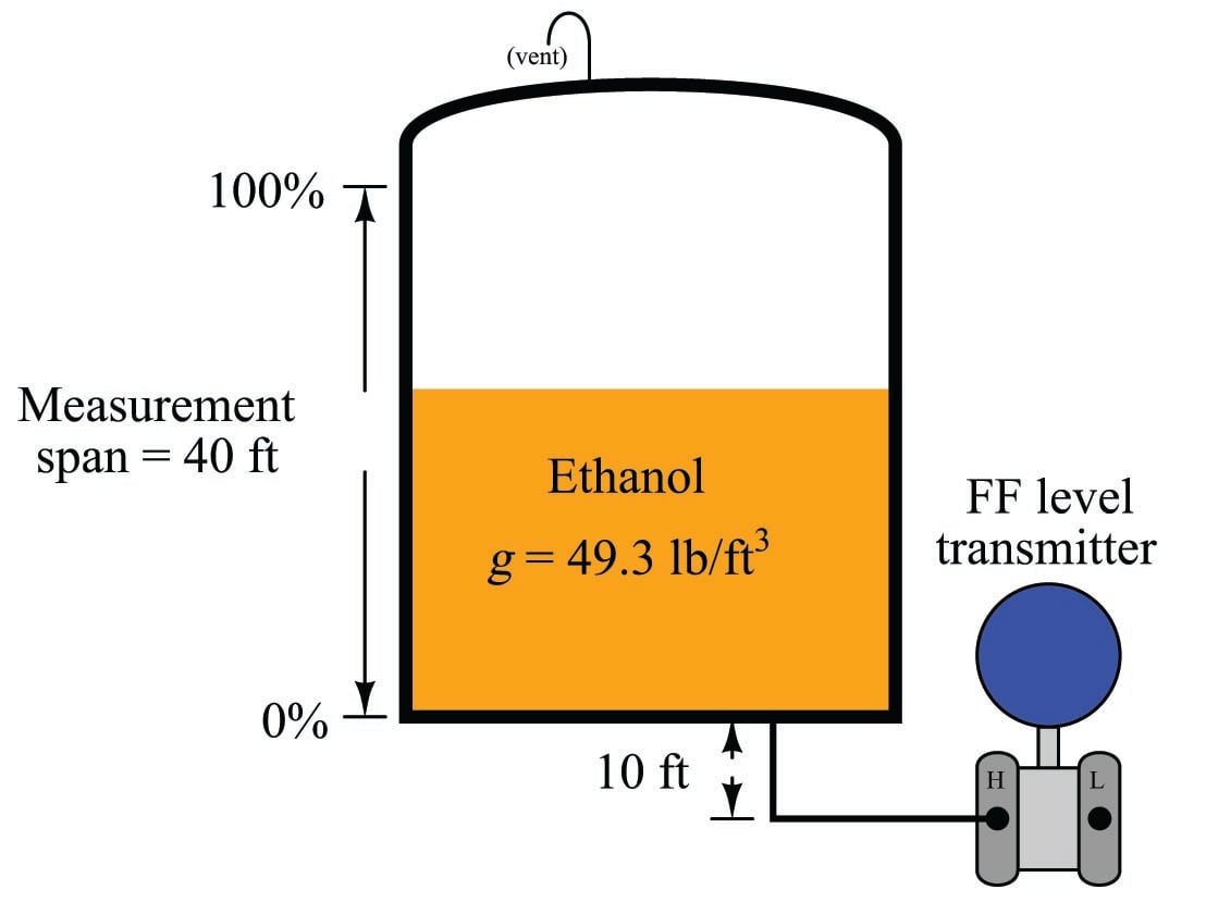
Hydrostatic pressure exerted on the transmitter’s sensing element is the product of liquid density (\(\gamma\)) and vertical liquid column height (\(h\)). When the tank is empty, there will still be a vertical column of ethanol 10 feet high applying pressure to the transmitter’s “high” pressure port. Therefore, the pressure seen by the transmitter in an “empty” condition is equal to:
\[P_{empty} = \gamma h_{empty} = (49.3 \hbox{ lb/ft}^3) (10 \hbox{ ft})\]
\[P_{empty} = 493 \hbox{ lb/ft}^2 = 3.424 \hbox{ PSI}\]
When the tank is completely full (40 feet), the transmitter sees a vertical column of ethanol 50 feet high (the tank’s 40 foot height plus the suppression height of 10 feet created by the transmitter’s location below the tank bottom). Therefore, the pressure seen by the transmitter in a “full” condition is equal to:
\[P_{full} = \gamma h_{full} = (49.3 \hbox{ lb/ft}^3) (40 \hbox{ ft} + 10 \hbox{ ft})\]
\[P_{full} = 2465 \hbox{ lb/ft}^2 = 17.12 \hbox{ PSI}\]
Thus, the transducer (XD) block in this Fieldbus transmitter will sense a liquid pressure ranging from 3.424 PSI to 17.12 PSI over the full range of the tank’s storage capacity.
However, we do not want this transmitter to publish a signal to the Fieldbus network in units of PSI, because the operations personnel monitoring this control system want to see a measurement of ethanol level inside the tank, not hydrostatic pressure at the bottom of the tank. We may be exploiting the principle of hydrostatic pressure to sense ethanol level, but we do not wish to report this measurement as a pressure.
The proper solution for this application is to set the L_Type parameter to “indirect” which will instruct the AI function block to mathematically scale the XD block’s pressure signal into a different range. Then, we must specify the expected pressure range and its corresponding level range as XD_Scale and OUT_Scale, respectively:
| AI block parameter | Range values |
|---|---|
| \texttt{L\_Type} | Indirect |
| \texttt{XD\_Scale} | 3.424 PSI to 17.12 PSI |
| \texttt{OUT\_Scale} | 0 feet to 40 feet |
Now, the ethanol tank’s level will be accurately represented by the FF transmitter’s output, both in numeric value and measurement unit. An empty tank generating a pressure of 3.424 PSI causes the transmitter to output a “0 feet” digital signal value, while a full tank generating 17.12 PSI of pressure causes the transmitter to output a “40 feet” digital signal value. Any ethanol levels between 0 and 40 feet will likewise be represented proportionally by the transmitter.
If at some later time the decision is made to re-locate the transmitter so it no longer has a 10 foot “suppression” with regard to the tank bottom, the XD_Scale parameters may be adjusted to reflect the corresponding shift in pressure range, and the transmitter will still accurately represent ethanol level from 0 feet to 40 feet, without re-calibrating or re-configuring anything else in the transmitter.
If we wished, we could even mathematically determine the liquid volume stored inside this ethanol tank at different sensed pressures, and then scale the AI block’s OUT_Scale parameter to report a volume in units of gallons, liters, cubic feet, or any other appropriate volume unit. Using the “indirect” mode with appropriate XD_Scale and OUT_Scale parameter values gives us great flexibility in how the transmitter senses and represents process data.
In summary, we set the XD_Scale parameter to the physical range of measurement directly sensed by the transducer, we set the OUT_Scale parameter to the corresponding range of measurement we wish the transmitter to report to the rest of the control system, and we set L_Type to “indirect” to enable this translation from one range to another. We should only use the “direct” L_Type setting if the raw transducer range is appropriate to output to the rest of the control system (e.g. if the transmitter directly senses fluid pressure and we wish this very same pressure value to be published onto the Fieldbus network by the transmitter, with no scaling).
Here is another Fieldbus transmitter ranging application, this time a differential pressure transmitter sensing pressure dropped across an orifice plate in order to infer the rate of flow for fluid inside the pipe. The transmitter senses small amounts of pressure difference (expressed in a unit of pressure called inches water column), but what we want it to report to the Fieldbus network is an actual flow rate in gallons per minute.
If we happen to know that this orifice plate produces a pressure drop of 125 inches water column (125 "WC) at a flow rate of 350 gallons per minute (350 GPM), we could set up the scaling parameters as shown:
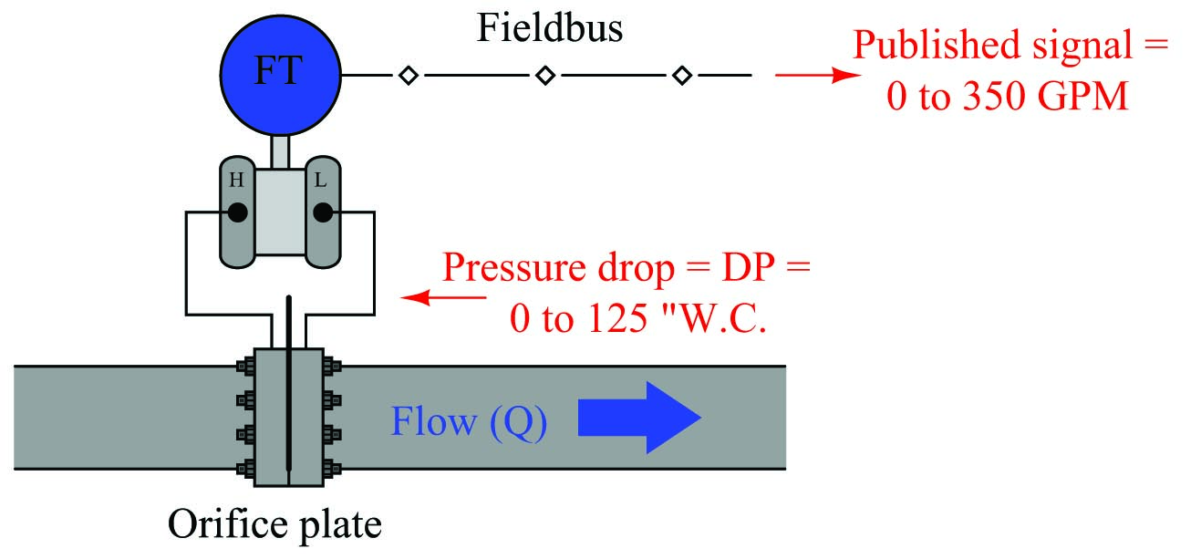
| AI block parameter | Range values |
|---|---|
| \texttt{L\_Type} | Indirect Square Root |
| \texttt{XD\_Scale} | 0 inches water to 125 inches water |
| \texttt{OUT\_Scale} | 0 GPM to 350 GPM |
Note the use of the “indirect square root” L_Type parameter value instead of just “indirect” as we used in the ethanol tank example. The square root function is necessary in this application because the relationship between differential pressure (\(\Delta P\)) and flow rate (\(Q\)) through an orifice is nonlinear, as described by the following formula:
\[Q = k \sqrt{\Delta P}\]
This particular nonlinearity is unique to pressure-based measurements of fluid flow, and does not find application in any other form of process measurement.
As before, though, we see a common theme with the XD_Scale and OUT_Scale parameter ranges: we set the XD_Scale parameter to the physical range of measurement directly sensed by the transducer, we set the OUT_Scale parameter to the corresponding range of measurement we wish the transmitter to report to the rest of the control system, and we set L_Type to “indirect” to enable this translation from one range to another.

Cool