Robot Kinematics

For engineers involved in the development of robot operating systems, there is an elevated level of understanding that goes into the mathematics of robot motion. Even for those not involved with OS programming, the knowledge of how a robot can coordinate the actions of 4-6 rotational joints and end up with linear motion at a precision of hundredths of millimeters is quite interesting.

What’s the End Goal of Robot Kinematics?

Before exploring some of the processes behind kinematic calculations, it’s always important to return back to why those formulas are being used in the first place.

It’s really a very simple goal: move the TCP from one spot to another spot with the right velocity.

In reality, that is much easier said than done, since we must consider not only the TCP itself but the orientation of each linkage along the way, since not every joint has infinite rotational limits. Some forward-thinking must be done to ensure that the planned motion path is possible.

One point that might surprise novice robot users is that, while a motion command may appear as a single line in a code, the motion is broken down into many discrete steps, each movement command to the servo motors causing a single tiny action, with the end of that action being the beginning point of the next action. In reverse kinetic equations, meaning the target location is the input parameter, and the motion command is the output, a 6-axis robot may calculate slightly different motions for two seemingly identical paths. Perhaps the payload increased, and as the robot slowed to a stop, the encoder attached to one of the joints stopped one click beyond the previous stopping point. This small change may lead to a slightly different calculation of the next step, progressing to a point where there may even be physical changes in the motion trajectory.

This is the reason for repeatability errors. How, if a robot is perfectly consistent, could the gripper land on a different spot each time the motion is performed? In theory, it should always follow the same path, but reality says otherwise.

Reverse Kinematics: Position

If we know the position of each motor and linkage in a 6-axis robot and its EoAT, we can piece together the vector sums in all 3 dimensions and arrive at the end coordinate of the TCP. Any rotational joint can cause a change of motion along a single plane. By itself, that single plane of motion is the plane normal to the axis around which it rotates, as can be seen in the following image.

In this image, the black dashed line shows the axis around which J5 (the wrist joint) rotates. Perpendicular, or ‘normal’, to that axis is the blue rectangular plane, which is actually infinite in size, although shown smaller here to give a perspective representation. As J5 rotates + and -, the final position of the TCP will change only along the blue plane, with an x and y positional change indicated by the two red arrows.

However, even though each joint can only change along two axes, the 6 joints all working together ensure that no joint can be considered in isolation.

From the image above, although J5 may only move in two dimensions, it should be fairly clear by mentally imagining the motion that jogging this joint will adjust the TCP in all three dimensions. J1 provides motion on the x-y plane, but all other joints past that point will distort the perfect alignment of the TCP along any axis. This provides incredible freedom of motion at the expense of a very tricky 3-dimensional kinematic calculation.

This all sounds very tricky to create a dynamic algorithm to handle, but the reality is that the problem is even more complicated than this. If the angle and linkage radius of all joints is known, there is a single unknown variable: the final TCP location. The robot, however, does not know the position of all joints in advance of a move, rather it is the opposite problem. Only one variable is known: the target coordinate of your motion command. The position of all joints is unknown and must be determined mathematically.

Kinematics in Joint Versus Linear Motion Commands

For any motion command with 6 axes of rotation, there would be a few ways to get from one point to another. In some cases, many ways. Robots are programmed to take advantage of the fastest joints to make the motion while minimizing deviation from the projected path. If a little bit of deviation is acceptable, such as a rapid transit from a conveyor on one side to another with no major obstacles, priority should be placed on speed over linearity of the move.

This rapid transit prioritizing speed and cycle time over accuracy is known as a ‘joint’ move. With careful observation (or simulation) tracking the TCP, you would see it moving in a slight arc motion, and that arc may change as the speed increases. Surprisingly, there may be a certain speed when one motor becomes more advantageous than another, and the entire path of motion will change as you increase the speed. This is why dry-run testing and accurate simulation is SO important to installation.

When you approach a final pick location or begin a weld pattern, this unpredictable arc motion is unacceptable. The movement of choice now becomes the ‘linear’ motion type. The speed and optimization of the move is now unimportant. The kinematic equations must ensure that each discrete servo command, down to the best accuracy of the robot, moves the TCP in a perfectly straight line.

Linear motion is by far the most predictable, but it should be used judiciously. Since it is far more restrictive in which motors can be used, it must often rely on slower motors, raising the time it takes to complete the move. ROI and cycle time are important in any process, so why not use the program commands for the reasons they were designed?

Reverse Kinematics: Velocity

Velocity is closely related to the position, but it does deserve its own discussion. In popular physics, the velocity is simply the discrete rate of change of the position, a derivative relationship. However, once again, the current velocity is always determined by the difference between the first and second position over the time between the two positions as the time approaches a nearly infinitely small duration. This is easy when the time and the positions are known and the velocity is the unknown variable, but we are faced once again with the dilemma that the velocity is the target input and the time and distance to move are both outputs to be sent from the controller to the servo motors.

Velocity is a particularly interesting property of kinematics because it has both a linear and angular element to the rotation, but the unit used in the command is simply the linear velocity, so both elements must be factored into the kinematics simultaneously. Position, by itself, is a coordinate suspended in time, with both an x-y-z center point and an angle (yaw, pitch and roll), so it also has different units. Usually, these are mm for the position, and degrees (sometimes radians) for the angle. Both the coordinate and the angle can be viewed for any position at any time.

However, when a linear command is entered into the code, the target speed is specified as a parameter, you can’t simply open a menu and view the current velocity of each axis and the rotation around each axis throughout the duration of the movement as you can with positional data. This causes velocity to be a bit of a mysterious player in the dynamic motion of the system.

Velocity has two unit systems, one for linear motion and the other for rotation.

Linear motion units may be selectable, but will most often be displayed as millimeters per second, mm/s. This speed is a very critical factor in collaborative robots since, according to the latest safety standards, the maximum linear speed of a collaborative robot cannot exceed the teaching speed of 250 mm/s, which is still quite fast.

The angular velocity of a joint will not provide any information on how fast the robot itself is moving, but rather, how fast the joints are rotating, in either degrees/s (deg/s) or radians/s (rad/s). To determine the actual speed of a point on the arm, the angular velocity must be multiplied by the radial arm distance to the next linkage. So although two robots may have identical angular velocities, the actual final travel speed of the tool will depend on the length of the linkages.

Coordinates and Velocities Vs. Joint Motions

One curious challenge in the programming of kinematic equations for robot motion is that the commands to the servos are entirely different from the two desired objectives of the motion of the end tool, those being the coordinates and the linear velocity of the tool.

When servo commands are issued, they are in the form of target positions in a certain timeframe. Attached to rotary encoders, the servos are told to advance or reverse by a certain number of degrees at a time, usually in fractions of degrees. The resolution of each command is defined by the incredibly high encoder resolutions (I have seen some servo motors rated with up to 32 million pulses per revolution!). This information sent to the servo always leads to motion in the form of degrees per second (ω), and, once the move is completed, a final angular position (θ).

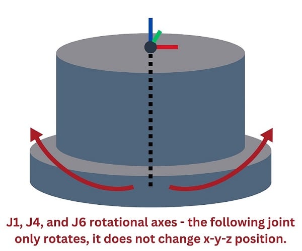
There are two types of rotary joints present on every 4 to 6-axis articulated arm robot. The first kind is always located at the base joint, and in 6-axis robots, it is also located at the 4th axis in the arm before the wrist, as well as the final 6th joint at the end of the wrist itself.

In this kind of joint, shown in the image below, the centerpoint of the following axis attachment point is located at a fixed point in space, but it is free to rotate around the axis of revolution. As you can visualize from the image, no matter how the joint rotates, the position of the colored XYZ coordinate indicator will not move, it will simply rotate. This is critical for the remaining joints along the arm, providing them with the ability to rotate in an arc around the base.

Some robot designs place the following joint at an offset distance from the axis of rotation, so those joints are more like a linkage and a traditional revolute joint. At the detriment of slightly more complex algorithms, the benefit is increased work area flexibility.

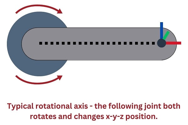
The other kind of joint, which is a more typical representation of a rotary joint, is shown in the image below. This is a motor attached to a linkage, forming the upper or lower arm of the articulated robot. This provides motion of the EoAT closer or away from the robot base, but without the rotation of the base (J1), the motion would not happen in 3D space around the robot. As you can visualize from the picture, as the servo rotates, the position of the colored XYZ indicator will move, and it will rotate as the motor spins.

Combining both types of joints in 4-6 axes, we can perform trigonometric calculations with both the velocity and the position in order to obtain the information about the tool center point. However, performing the inverse trigonometric calculations should simply work this process in revers, the only problem is that, in many cases, there are multiple configurations to reach the exact same point. Most of the time, this only creates problems in the inability to predict exactly what motion path will be chosen by the controller from point A to B.

Singularity - What Is It and How Do You Fix It?

Some of these multiple motion path problems are unsolvable, with one particular situation referred to as a point of ‘singularity’. Many robotic engineers have faced this problem, but far fewer understand what it means and why it’s such a big problem.

When the robot arm is extended to its furthest reach, or at least the last few joints are stretched out as far as the tool can reach, those joints form a perfectly straight line from the elbow joint (usually J3) all the way to the end face of the arm.

The robot in the image below is not exactly in the singularity position (fortunately for the operator) but if joint 5 is jogged about 30 degrees up to put the end of the arm in alignment, then the error might occur.

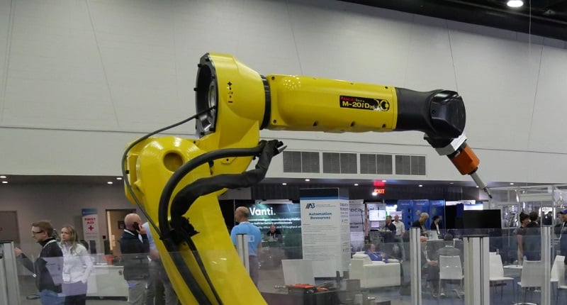
Since both J4 and J6 provide the same revolution about the same axis when aligned like this, there are an infinite number of possible solutions to get the robot to extend in the Z-direction (normal to that end face) Think about it this way, J4 could rotate a few degrees in the positive direction, while J3 rotates equally in the opposite direction, or vise versa, or any other number of infinite possibilities. Because the robot is designed to calculate the shortest path, and there are infinitely possible solutions, the robot refuses to produce a meaningful output. Action will stop, the motors will be disabled, and a ‘singularity’ error will be displayed on the software.

This is likely to happen under two circumstances.

First, this can happen while teaching. The robot is being jogged in joint mode, the user has lined up the end joints in the arm, then switches to tool coordinate system and attempts to jog in the Z-direction. For context, imagine a CNC machine loading program and the robot has picked up the metal block and is approaching the vice jaws in a straight line.

The second scenario might occur during one of the first few times a program is tested at a certain speed. In order to get from point A to point B, the robot calculates a path. That path causes the robot to align the end joints, which is more or less a coincidence. The fault will suddenly occur mid-transit and shut down operations.

The worst part about this second scenario is that it may not happen the first, second, or more times the routine is run. There may be some specific set of conditions under which it happens once, and is hard to replicate. The error, confusing enough by itself, is harder to understand being difficult to repeat.

How then, do we solve this problem?

If the error occurs during jogging in teach mode, it can be solved by moving the wrist joint up or down slightly, just a few degrees. The error will never appear in joint jogging mode, so you can clear the error, then jog the wrist joint (J5 in a 6-axis robot) + or - just a few degrees, then continue jogging as before.

If the error occurs during a running program, first, try to identify the closest points between which the error occurred (call them points A and B). The good news is that it doesn’t need to be exact, but try and figure out where the error occurred. Jog the robot to that point, then jog J5 + or - a few degrees, then save the point as a waypoint in the program. The waypoint motion command should be placed in the middle between those two points at which the error occurs. In other words, the new waypoint command should be placed right between point A and point B.

For this waypoint, it will be most productive to set the point termination of this new command to a continuous path, so that it does not stop momentarily on the point before continuing. Even with the continuous path, the altered joint orientation will still avoid the singularity problem, but it should not increase the cycle time very much. Perhaps a small increase is inevitable, but a fractional percent increase in cycle time is far superior to intermittent faults causing mysterious downtime events!

7th Axis Options

A final kinematic consideration in articulated arm design is how to add new features, such as a 7th axis. There are several designs I have seen for such an addition.

Sliding Axis

First, the robot can be mounted to a long, sliding axis, allowing a single robot to handle numerous tasks on an assembly line. This new axis is not particularly difficult to add into the control software, since it will likely alight with the X or Y axis, and therefore the position measured by the linear axis is simply added to the X or Y coordinate of the tool.

Adjustable Mounting Column

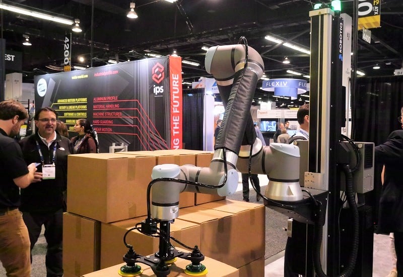
A similar sliding axis can be used in palletizing applications where the robot is mounted to the top or side of a vertical column axis. As the column is extended, the robot can stack higher. This motion is in the Z-direction, so a vertical axis will always add or subtract from the Z position of the TCP. Again, very simple to integrate into the programming.

Added Tool or Hand Axis

A 7th axis can also be built into the EoAT by the engineer, or added to the robot right at the wrist by the manufacturer. Both of these will create a slightly more difficult programming scenario because the TCP is not guaranteed to be aligned with the base coordinate system at all times. Nearly any sliding or rotary motion of an axis near the tool will cause motion in all three axes unless, by coincidence, the tool is aligned with the base coordinate system.

Future Robot Kinematics

As we know, predicting the future of technology is an exercise only in speculation. Who knows how we might be able to track motion more accurately, or if the current methods will always prevail? A possible option parallels the way in which a UAV (drone) tracks position, with its ability to monitor every motion down to the order of fractions of mm with a 9-axis motion sensor. If this was placed in the end tool, along with a power source, could it be accurate enough to place the end tool with utmost accuracy? Who knows how future automation will advance, but we know for sure that robotics will continue to become more driven by data, more precise and accurate, and safer with every passing leap of technology.