 Facebook
 Google
 GitHub
 Linkedin
Digital Data Communication Theory
One of the great benefits of digital technology is the ability to communicate vast amounts of information over networks. This very textbook you are reading was transmitted in digital form over the electronic network we call the Internet: a feat nearly impossible with any sort of analog electronic technology. The main benefit of digital data communication in industrial control is simple: no longer must we dedicate a single pair of wires to each and every variable we wish to measure and control in a facility as is necessary with analog (4-20 mA) signaling. With digital signaling, a single pair of wires or coaxial cable is able to convey a theoretically unlimited number of data points.
This benefit comes at a price, though: in order to communicate multiple variables (data points) over a single channel (wire pair), we must transmit and receive those signals one at a time. This means a digital communications system will necessarily exhibit some degree of time delay in acquiring, transmitting, receiving, and interpreting a signal. Analog systems, by contrast, are virtually instantaneous. Thus, we see a contrast between analog and digital communication pitting channel capacity against speed:
| Analog | Digital |
|---|---|
| Only one signal per channel | Many signals per channel possible |
| Instantaneous | Time-delayed |
With modern electronic technology it is possible to build digital communication systems that are so fast, the time delays are negligible for most industrial processes, which renders the second comparison (instantaneous versus time-delayed) moot. If time is no longer an issue, the advantage that digital communication has over analog in terms of channel usage makes it the superior choice.
Another important advantage of digital data communication for industrial processes is increased noise immunity. Analog data is continuous by nature: a signal of 11.035 milliamps has a different meaning than a signal of 11.036 milliamps, because any measurable increment in signal represents a corresponding increment in the physical variable represented by that signal. A voltage value in a 0-5 volt digital signaling system of 0.03 volts, however, means the exact same thing as a voltage value of 0.04 volts: either one is still interpreted as a “0” or “low” state. Any amount of electrical noise imposed on an analog signal corrupts that signal to some degree. A digital signal, however, may tolerate a substantial amount of electrical noise with no corruption whatsoever.
Not surprisingly, though, the noise immunity enjoyed by digital signals comes with a price: a sacrifice in resolution. Analog signals are able to represent the smallest imaginable changes because they are continuously variable. Digital signals are limited in resolution by the number of bits in each data “word.” Thus, we see another contrast between analog and digital data representation:
| Analog | Digital |
|---|---|
| Corrupted by any amount of noise | Immune to certain (limited) amounts of noise |
| Unlimited resolution | Limited resolution |
With modern digital electronic technology, however, the “limited resolution” problem is almost nonexistent. 16-bit converter chipsets are commonly available today for input/output (I/O) modules on digital systems, providing a resolution of \(2^{16}\) (65536) counts, or \(\pm\) 0.00153%, which is good enough for the vast majority of industrial measurement and control applications.
This section will focus on serial data transmission, as opposed to parallel. In order to transmit digital data in parallel form, the number of wires scales directly with the number of bits in each data “word.” For example, if a 16-bit ADC chip were to communicate its data to some other digital device using a parallel network, it would require a cable with 16 wires (plus a common “ground” wire) at minimum. Since this approach undercuts the “fewer wires” advantage that digital communications theoretically enjoys over analog communication, parallel data transmission is rarely seen in industry except for within the internal construction of a digital device (e.g. a parallel data bus inside a personal computer, or inside a PLC or DCS rack).
In serial communications systems, digital data is sent over a wire pair (or fiber optic cable, or radio channel) one bit at a time. A 16-bit digital “word” (two bytes in length) then will require a succession of 16 bits transmitted one after the other in time. How we represent each bit as an electrical signal, how we arrange those bits in time to group them into meaningful “words,” and how multiple devices share access to a common communications channel, is our next subject of exploration: the technical details of serial data communication.
Serial communication principles
The task of encoding real-life data as a series of on-and-off electrical signals, and then sending those signals long distances over electrical cables (or optical fibers, or radio waves) requires mutually-agreed standards for the encoding, the “packaging” of those bits, the speed at which the bits are sent, methods for multiple devices to use a common channel, and a host of other concerns. This subsection will delineate the major points of compatibility necessary for digital devices to communicate serially. We begin with a brief exploration of some of the standards used in early telegraph systems.
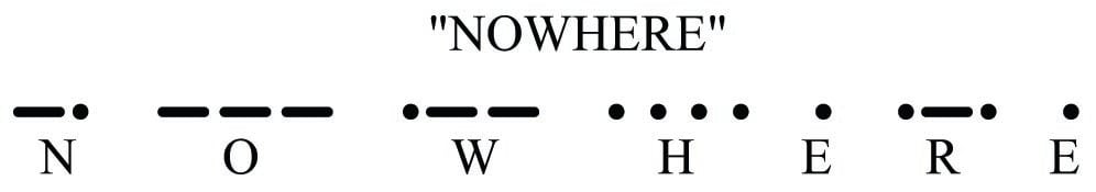
An early form of digital communication was Morse Code, used to communicate alpha-numerical information as a series of “dots” and “dashes” over telegraph systems. Each letter in the alphabet, and each numerical digit (0 through 9) was represented in Morse Code by a specific series of “dot” and “dash” symbols, a “dot” being a short pulse and a “dash” being a longer pulse. A similar code system called the Continental Code was used for early radio (“radiotelegraph”) communications.
As primitive as these codes were, they encapsulated many of the basic principles we find in modern digital serial communication systems. First, a system of codes was necessary in order to represent English letters and numerals by electrical pulses. Next, there needed to be some way to delineate the beginning and end of each character.
For example, consider the Continental Code encoding for the word NOWHERE. By placing an extra space (a pause in time) between characters, it is easy to represent individual characters in the message:
If this space between characters were not present, it would be impossible to determine the message with certainty. By removing the spaces, we find multiple non-sensical interpretations are possible for the same string of “dots” and “dashes:”
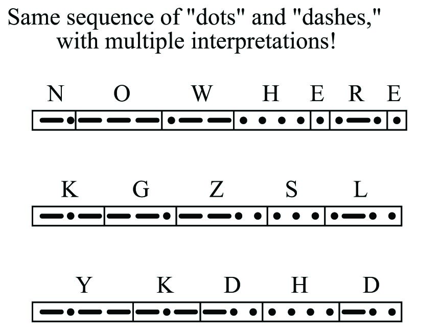
For that matter, it is even possible to confuse the meaning of the text string “NOWHERE” when the individual characters are properly interpreted. Does the string of characters say “NOWHERE,” or does it say “NOW HERE”?
This simple example illustrates the need for delimiting in serial data communication. Some means must be employed to distinguish individual groups of bits (generally called frames or packets) from one another, lest their meanings be lost. In the days when human operators sent and interpreted Morse and Continental code messages, the standard delimiter was an extra time delay (pause) between characters, and between words. This is not much different from the use of whitespace to delineate words, sentences, and paragraphs typed on a page. Sentenceswouldcertainlybeconfusingtoreadifnotforspaces!
In later years, when teletype machines were designed to replaced skilled Morse operators, the concept of frame delineation had to be addressed more rigorously. These machines consisted of a typewriter-style keyboard which marked either paper strips or pages with dots corresponding to a 5-bit code called the Baudot code. The paper strip or sheets were then read electrically and converted into a serial stream of on-and-off pulses which were then transmitted along standard telegraph circuit lines. A matching teletype machine at the receiving end would then convert the signal stream into printed characters (a telegram). Not only could unskilled operators use teletype machines, but the data rate far exceeded what the best human Morse operators could achieve. However, these machines required special “start” and “stop” signals to synchronize the communication of each character, not being able to reliably interpret pauses like human operators could.
Interestingly, modern asynchronous serial data communication relies on the same concept of “start” and “stop” bits to synchronize the transmission of data packets. Each new packet of serial data is preceded by some form of “start” signal, then the packet is sent, and followed up by some sort of “stop” signal. The receiving device(s) synchronize to the transmitter when the “start” signal is detected, and non-precision clocks keep the transmitting and receiving devices in step with each other over the short time duration of the data packet. So long as the transmitting and receiving clocks are close enough to the same frequency, and the data packet is short enough in its number of bits, the synchronization will be good enough for each and every bit of the message to be properly interpreted at the receiving end.
Physical encoding of bits
Telegraph systems were Boolean in nature: representing “dots” and “dashes” by one electrical state of the telegraph line, and pauses by another. When manually-actuated keyswitches were abandoned in favor of teletype machines, and Morse code abandoned in favor of the Baudot (5-bit) code for representing alphanumeric characters, the electrical nature of the telegraph (at least initially) remained the same. The telegraph line would either be energized or not, corresponding to marks or spaces made on the teletype paper.
Many modern digital communication standards represent binary “1” and “0” values in exactly this way: a “1” is represented by a “mark” state and a “0” is represented by a “space” state. “Marks” and “spaces” in turn correspond to different voltage levels between the conductors of the network circuit. For example, the very common EIA/TIA-232 serial communications standard (once the most popular way of connecting peripheral devices to personal computers, formerly called RS-232) defines a “mark” (1) state as \(-3\) volts between the data wire and ground, and a “space” (0) state as +3 volts between the data wire and ground. This is referred to as Non-Return-to-Zero or NRZ encoding:
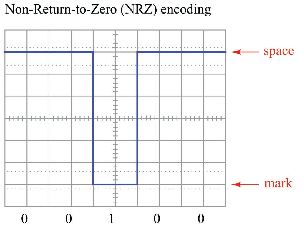
An easy way to remember the difference between a “mark” and a “space” in this scheme is to recall the operation of old telegraph printing units, specifically how they created marks and spaces on moving paper strip. When the printing unit was energized (i.e. the transmitting key was pressed, sending current through the solenoid coil of the printer, corresponding to a “1” state), the printer’s iron armature would be pulled down to draw a mark on the paper strip. When de-energized (transmitting key released, stopping current in the telegraph line, corresponding to a “0” state), the printer’s armature would spring-return up from the paper to leave a blank space.
This is not the only way to represent binary bits, though. An alternative method is to use an oscillating (square-wave) signal, counting up and down transitions (pulse edges) at specific times to represent 1 and 0 states. This is called Manchester encoding, and it is used in the 10 Mbps (10 million bits per second) version of Ethernet and in both the FOUNDATION Fieldbus “H1” and Profibus “PA” instrumentation network standards:

Note how each binary bit (0 or 1) is represented by the direction of the voltage signal’s transition. A low-to-high transition represents a “1” state while a high-to-low transition represents a “0” state. Extra “reversal” transitions appear in the pulse stream only to set up the voltage level as needed for the next bit-representing transitions. The representation of bits by transitions rather than by static voltage levels guarantees the receiving device can naturally detect the clock frequency of the transmitted signal. Manchester data is therefore referred to as self-clocking.
Interpreting a Manchester waveform is easier than it first appears. The key is identifying which transitions represent “clocked” bits and which transitions represent “reversals” prior to bits. If we identify the widest periods of the waveform, we know the transitions in these periods must represent real bits because there are no reversals. Another way to say this is the greatest time period found between successive transitions in a Manchester waveform is the clock period. Once we identify this clock period, we may step along the waveform at that same period width to distinguish clocked bits from reversals.
Yet another method for encoding binary 1 and 0 states is to use sine waves of different frequencies (“tone bursts”). This is referred to as Frequency Shift Keying, or FSK, and it is the method of encoding used in the HART “smart” instrument communications standard.
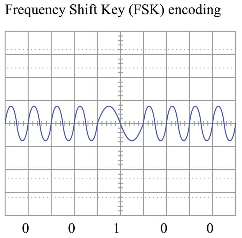
In the HART standard – based on the Bell 202 standard used in telephone data exchange – two complete cycles at 2200 Hz represents a “0” bit (space), while one complete cycle at 1200 Hz represents a “1” bit (mark). This standard was invented as a way to exchange digital data over telephone networks, which were built to communicate audio-frequency AC signals and thus could not reliably communicate the square-wave signals associated with direct digital data. By assigning digital values to different audio frequencies, serial data could be communicated over telephone channels as a series of sine-wave tones.
The same principle of FSK allows HART-compatible instruments to communicate digital data over cables simultaneously carrying DC current (4 to 20 mA) signals representing control system data. Since each bit of FSK-encoded data consists of complete AC cycles (one full positive swing for every full negative swing), the superposition of AC tones does not affect the time-averaged value of the DC milliamp signal.
Other methods exist as well for encoding digital data along network cables, but these three are the most popular in industrial networks.
Communication speed
In order to successfully communicate digital data along a network, there must not only be a standard agreed upon between transmitting and receiving devices for encoding bits (NRZ, Manchester, FSK, etc.), but there must also be a standard in place for the speed at which those bits will be sent. This is especially true for NRZ and FSK encoding, where the “clock” speed is not explicitly present in the signal.
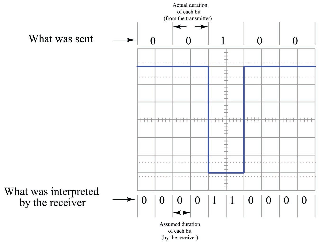
For example, consider the confusion that could arise interpreting a NRZ signal if the transmitting device sends data at half the speed assumed by the receiving device:
Thus, one of the essential parameters in a serial data communication system is the bit rate, measured in bits per second (bps). Some communications standards have fixed bit rates, such as FOUNDATION Fieldbus H1 and Profibus PA, both standardized at exactly 31.25 kbps. Some, such as Ethernet, have a few pre-defined speeds (10 Mbps, 100 Mbps, 1 Gbps) defined by the specific transmitting and receiving hardware used. Others, such as EIA/TIA-232 may be arbitrarily set by the user at speeds ranging from 300 bps to over 115 kbps.
An older term sometimes used synonymously with bit rate is baud rate, however “bits per second” and “baud” are actually different things. “Baud” refers to the number of voltage (or current) alternations per second of time, whereas “bits per second” refers to the actual number of binary data bits communicated per second of time. Baud is useful when determining whether or not the bandwidth (the maximum frequency capacity) of a communications channel is sufficient for a certain communications purpose. For a string of alternating bits (e.g. 010101010101) using NRZ encoding, the baud rate is equivalent to the bit rate: exactly one voltage transition for each bit. For a string of unchanging bits (e.g. 000000000000 or 111111111111) using NRZ encoding, the baud rate is far less than the bit rate. In systems using Manchester encoding, the worst-case baud rate will be exactly twice the bit rate, with two transitions (one up, one down) per bit. In some clever encoding schemes, it is possible to encode multiple bits per signal transition, such that the bit rate will actually be greater than the baud rate.
Data frames
As mentioned earlier in this section, serial data is usually communicated asynchronously in industrial networks. This means the transmitting and receiving hardware need not be in perfect synchronization to reliably send and receive digital data. In order for this to work, data must be sent in “frames” or “packets” of fixed (maximum) length, each frame preceded by a special “start” signal and concluded with a special “stop” signal. As soon as the transmitting device issues the “start” signal, the receiving device synchronizes to that start time, and runs at the pre-determined clock speed to gather the successive bits of the message until the “stop” signal is received. So long as the internal clock circuits of the transmitting and receiving devices are running at approximately the same speed, the devices will be synchronized closely enough to exchange a short message without any bits being lost or corrupted. There is such a thing as a synchronous digital network, where all transmitting and receiving devices are locked into a common clock signal so they cannot stray out of step with each other. The obvious advantage of synchronous communication is that no time need be wasted on “start” and “stop” bits, since data transfer may proceed continuously rather than in packets. However, synchronous communication systems tend to be more complex due to the need to keep all devices in perfect synchronization, and thus we see synchronous systems used for long-distance, high-traffic digital networks such as those use for Internet “backbones” and not for short-distance industrial networks.
Like bit rate, the particular scheme of start and stop bits must also be agreed upon in order for two serial devices to communicate with each other. In some networks, this scheme is fixed and cannot be altered by the user. Ethernet is an example of this, where a sequence of 64 bits (an alternating string of “1” and “0” bits ending with a “1, 1”; this is the “preamble” and “start frame delimiter” or “SFD” bit groups) is used to mark the start of a frame and another group of bits specifies the length of the frame (letting the receiver know ahead of time when the frame will end). A graphic description of the IEEE 802.3 standard for Ethernet data frames is shown here, illustrating the lengths and functions of the bits comprising an Ethernet frame:

Other serial networks offer choices for the user to select regarding these parameters. One such example is EIA/TIA-232, where the user may specify not only the bit rate, but also how many bits will be used to mark the end of the data frame. It is imperative in such systems that all transmitting and receiving devices within a given network be configured exactly the same, so that they will all “agree” on how to send and receive data. A screenshot from a UNIX-based serial communication terminal program (called minicom) shows these options:
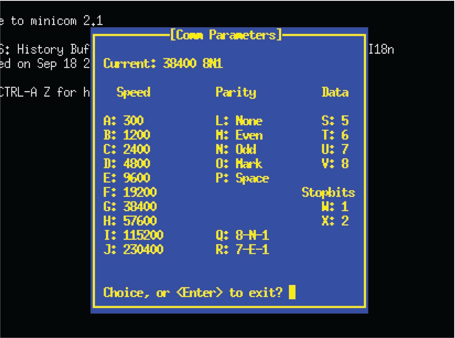
In this particular screenshot, you can see the data rate options (extending from 300 bps all the way up to 230400 bps!), the number of data bits (from 5 to 8), and the number of stop bits (1 or 2), all configurable by the user. Of course, if this program were being used for communication of data between two personal computers, both of those computers would need these parameters set identically in order for the communication to take place. Otherwise, the two computers would not be in agreement on speed, number of data bits, and stop bits; their respective data frames simply would not match.
To give an example of an EIA/TIA-232 data frame might look like as a series of voltage states, consider this waveform communicating a string of eight bits (01011001), using NRZ encoding. Here, a single “start” marks the beginning of the data frame, while two successive “stop” bits end it. Also note how the bit sequence is transmitted “backwards,” with the least-significant bit (LSB) sent first and the most-significant bit (MSB) sent last:

Interestingly, the “mark” state (corresponding to a binary bit value of “1”) is the default state of the communications channel when no data is being passed. The “start” bit is actually a space (0). This is the standard encoding scheme for EIA/TIA-232, EIA/TIA-485, and some other NRZ serial communication standards.
One of the options you probably noticed in the “minicom” terminal program screenshot was something called parity. This is a simple form of error-checking used in many serial communication standards. The basic principle is quite simple: an extra bit is added at the end of the data frame (between the data and stop bits) to force the total number of “1” states to be either odd or even. For example, in the data stream just shown (10011010), there is an even number of “1” bits. If the serial device sending this eight-bit data group were configured for “odd” parity, it would append an additional “1” to the end of that frame to make the total number of “1” bits odd rather than even. If the next data group were 11001110 instead (already having an odd number of “1” bits), the transmitting device would have to attach a “0” parity bit on to the data frame in order to maintain an odd count of “1” bits.
Meanwhile, the receiving device is programmed to count up all the “1” bits in each data frame (including the parity bit), and check to see that the total number is still odd (if the receiving device is configured for odd parity just as the transmitting device, which the two should always be in agreement). Unlike the transmitting device which is tasked with creating the parity bit state, the receiving device is tasked with reading all the data bits plus the parity bit to check if the count is still as it should be. If any one bit somehow gets corrupted during transmission, the received frame will not have the correct parity, and the receiving device will “know” something has gone wrong. Parity does not suggest which bit got corrupted, but it will indicate if there was a single-bit corruption of data, which is better than no form of error-checking at all.
The following example shows how parity-checking would work to detect a transmission error in a 7-bit data word. Suppose a digital device asynchronously transmits the character “T” using ASCII encoding (“T” = 1010100), with one start bit, one stop bit, and “odd” parity. Since the “start” bit is customarily a 0 state (space), the data transmitted in reverse order (LSB first, MSB last), the parity bit transmitted after the data’s MSB, and the “stop” bit represented by a 1 state (mark), the entire frame will be the following sequence of bits: 0001010101. Viewed on an oscilloscope display where a negative voltage represents a “mark” and a positive voltage represents a “space,” the transmitted data frame will look like this:
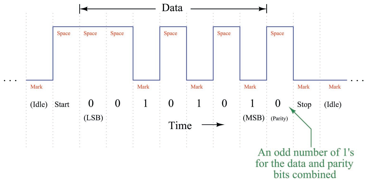
Note how the parity bit in this particular frame has been generated by the transmitting device as a 0 state, because the parity type is set for “odd,” and the transmitting device realizes that the 7-bit data word already has an odd number of 1 bits in it and doesn’t need another “1” for the parity bit. The pulse waveform you see above is how this data frame will be transmitted onto the network.
Now suppose this transmitted frame encounters a significant amount of electrical noise as it travels to the receiving device. If the frame reaches the receiver as shown in the next illustration, the receiving device will interpret the message incorrectly:

One of the bits has been corrupted by noise, such that the fifth transmitted data bit (which should be 1) is instead received as a 0. The receiving device, of course, has no knowledge of the noise present on the NRZ signal because all it “sees” is the “mark” or “space” states as interpreted by its input buffer circuitry. When the receiving device goes to count the number of 1 bits in the message (data plus parity bit, disregarding start and stop bits), however, it will count an even number of 1’s instead of an odd number of 1’s. Since the receiving device is also set for “odd” parity to match the transmitting device, it expects an odd number of 1’s in the received message. Thus, it “knows” there is a problem somewhere in this transmission, because the received parity is not odd as it should be.
Parity-checking does not tell us which bit is corrupted, but it does indicate that something has gone wrong in the transmission. If the receiving device is programmed to take action on receipt of a non-matching parity, it may reply with a request for the transmitting device to re-send the data as many times as necessary until the parity is correct.
If we look at the “minicom” terminal screenshot again to analyze the parity options, we see there are several to choose from:
The five options for parity in this program include None, Even, Odd, Mark, and Space. “No” parity is self-explanatory: the transmitting device does not attach an extra bit for parity at all, and the receiving device does not bother to check for it. Since the inclusion of a parity bit does add to the bulk of a data frame, it has the unfortunate effect of slowing down communications (more bit “traffic” occupying the channel than would otherwise need to be), thus the option to waive parity altogether for a more compact (faster) data frame. “Even” and “Odd” parity options work as previously described, with the transmitting device adding a parity bit to each frame to bring the total “1” bit count either to an even number or to an odd number (depending on the user’s configuration), and the receiving device checks for the same. “Mark” and “Space” are really of limited usefulness. In either of these two options, a parity bit is added, but the transmitting device does not bother to calculate the evenness or oddness of the data bits, rather simply making the parity bit always equal to 1 (“mark”) or 0 (“space”) as chosen by the user. The receiving device checks to see that the parity bit is always that value. These two options are of limited usefulness because the parity bit fails to reflect the status of the data being transmitted. The only corruption the receiving device can detect, therefore, is a corruption of the parity bit itself!
One will often find the communications parameters of a serial network such as this displayed in “shorthand” notation as seen at the top of the “minicom” terminal display: 38400 8N1. In this case, the terminal program is configured for a bit rate of 38400 bits per second, with a data field 8 bits long, no parity bit, and 1 stop bit. A serial device configured for a bit rate of 9600 bps, with a 7-bit data field, odd parity, and 2 stop bits would be represented as 9600 7O2.
Parity bits are not the only way to detect error, though. Some communication standards employ more sophisticated means. In the Ethernet (IEEE 802.3) standard, for example, each data frame is concluded with a frame check sequence, which is a collection of bits mathematically calculated by the transmitting device based on the content of the data. The algorithm is called a cyclic redundancy check, or CRC, and is similar to the concept of “checksum” used by computers to check the integrity of data stored in hard disks and other “permanent” media. Like a parity algorithm, the CRC algorithm runs through a mathematical process whereby all the bits in the data field are counted, and a number is generated to reflect the statuses of those bits. The receiving device takes the received data field and performs the exact same mathematical algorithm, generating its own CRC value. If any of the data’s bits become corrupted during transmission, the two CRC values will not match, and the receiving device will know something has gone wrong.
Like parity, the CRC algorithm is not perfect. There exists a chance that just the right combination of errors may occur in transmission causing the CRC values at both ends to match even though the data is not identical, but this is highly unlikely (calculated to be one chance in \(10^{14}\)). It is certainly better than having no error detection ability at all.
If the communications software in the receiving device is configured to take action on a detection of error, it may return a “request for re-transmission” to the transmitting device, so the corrupted message may be re-sent. This is analogous to a human being hearing a garbled transmission in a telephone conversation, and subsequently requesting the other person repeat what they just said.
Another option often found in serial data communications settings is something called flow control, not to be confused with the actual control of fluid through a pipe. In the context of digital communications, “flow control” refers to the ability of a receiving device to request a reduction in speed or even a complete cessation of data transmission if the speed of the transmitted data is too fast for the receiving device to keep pace. An example common to personal computers is that of a mechanical printer: while the computer may be able to transmit data to be printed at a very rapid pace, the printer is limited by the speed of its printing mechanism. In order to make the printing process go more smoothly, printers are equipped with buffer memory to store portions of the print job received from the transmitting computer that have not had time to print yet. However, these buffers are of finite size, and may become overwhelmed on large print jobs. So, if and when a printer detects its buffer near full capacity, it may issue a command to the computer to freeze serial data transmission until the printer’s buffer has had some time to empty. In other words, the printer can send a message to the computer saying “Stop!” when its buffer is full, then later send another message saying “Resume” when its buffer is empty enough to resume filling. Thus, the receiving device has control over the flow of data necessary to manage its buffer resources.
Flow control in serial networks may take place in either hardware mode or software mode. “Hardware” mode refers to the existence of additional connector pins and cable conductors specifically designated for such “halt” and “resume” signals. “Software” mode refers to data codes communicated over the regular network channel telling the transmitting device to halt and resume. Software flow control is sometimes referred to as XON/XOFF in honor of the names given to these codes. Hardware flow control is sometimes referred to as RTS/CTS in honor of the labels given to the serial port pins conveying these signals.
The following screen shot shows options for flow control in the “minicom” terminal program:
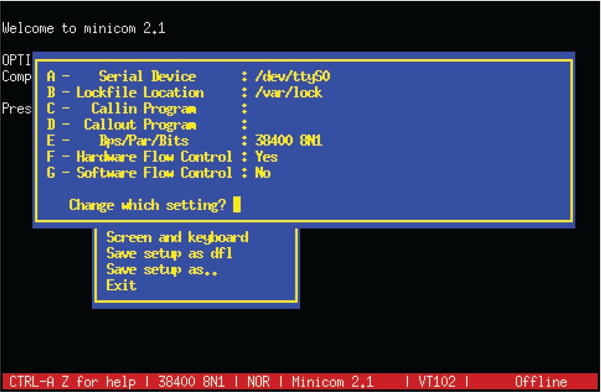
Here, you can see “hardware” flow control enabled and “software” flow control disabled. The enabling of “hardware” flow control means the serial communications cable must be equipped with the necessary lines to convey these handshaking signals (when needed) between devices. Software flow control tends to be the more popular option, the advantage of this of course being fewer conductors necessary in the serial data cable. The disadvantage of using software flow control over hardware is a slight inefficiency in data throughput, since the XON and XOFF commands require time to be transmitted serially over the same network as the rest of the data.
Channel arbitration
When two or more communication devices exchange data, the directions of their communication may be classified into one of two categories: simplex or duplex. A “simplex” network is one-way communication only. A sensor outputting digital data to a remotely-located indicator over a digital network would be an example of simplex communication, where the flow of information goes from sensor to indicator, and never the other direction. A public-address (PA) system is an analog example of a simplex communication system, since audio information only goes in one direction (from the person with the microphone to the audience).
“Duplex” communication refers to two-way data exchange. Voice telephony is an analog example of two-way (duplex) communication, where either person at the end of the connection can hear the other person talking. Duplex communication may be further subdivided into half-duplex and full-duplex, referring to whether or not the two-way communication may be simultaneous. In a “full-duplex” system, both devices may transmit data to each other simultaneously because they have separate channels (separate wires, or optical fibers, or radio frequencies) for their respective transmissions. In a “half-duplex” system, only one device may transmit at any time because the devices must share a common channel. A telephone system is an example of a full-duplex system, although it may be rather difficult for the people to understand each other when they are speaking over one another. A push-to-talk radio system (“walkie-talkie”) is an example of a half-duplex system, where each person must take turns talking.
Most industrial data networks are half-duplex, if only for the reason that most networks consist of more than two devices on a network segment. When more than two devices share a network, there are not enough data channels to allow all of the devices to simultaneously transmit and listen to each other. Thus, virtually any network supporting more than two devices will be half-duplex at best, and may even be limited to simplex operation in some cases.
In half-duplex systems, there must be some way for the respective devices to “know” when they are allowed to transmit. If multiple devices sharing one communications channel attempt to transmit simultaneously, their messages will “collide” in such a way that no device on the network will be able to interpret either message. The problem is analogous to two people simultaneously pressing the “talk” buttons on their two-way radio units: neither of the talking people can hear each other, and anyone else on the same channel hears the garbled amalgam of those two peoples’ superimposed transmissions. In order to avoid this scenario in a half-duplex network, there must be some strategy to coordinate transmissions so only one device “talks” at any given time. The problem of deciding “who” gets to “talk” at any given time is generally known as channel arbitration. Several strategies for addressing this problem have been developed in the data communications field, a few of which will be described in this subsection.
Master-slave
Our first method works on the principle of having only one device on the network (the “master”) with permission to arbitrarily transmit data. All other devices on the network are “slaves,” which may only respond in direct answer to a query from the master. If the network happens to be simplex in nature, slave devices don’t even have the ability to transmit data – all they can do is “listen” and receive data from the one master device.
For example, in a half-duplex master-slave network, if one slave device has data that needs to be sent to another slave device, the first slave device must wait until it is prompted (“polled”) by the master device before it is allowed to transmit that data to the network. Once the data is transmitted, any and all slave devices may receive that transmission, since they all “listen” to the same communications channel.
An example of an industrial network using master-slave channel arbitration is HART multidrop, where multiple HART field instruments are parallel-connected on the same wire pair, and one device (usually a dedicated computer) serves as the master node, polling the field instruments one at a time for their data.
Another example of a master-slave industrial network is a Modbus network connecting a programmable logic controller (PLC) to multiple variable-frequency motor drives (VFDs). The master device (the PLC) initiates all communications, with the slave devices (the motor drives) at most replying to the PLC master (and in many cases not replying at all, but merely receiving data from the PLC in simplex mode).
Master-slave arbitration is simple and efficient, but suffers from one glaring weakness: if the master device happens to fail, all communication on the network halts. This means the ability of any device on the network to transmit information utterly depends on the proper function of one device, representing a high level of dependence on that one (master) device’s function.
Some master-slave networks address this problem by pre-assigning special “back-up” status to one or more slave devices. In the event that the master device fails and stops transmitting for a certain amount of time, the back-up device becomes “deputized” to act as the new master, taking over the role of the old master device by ensuring all slave devices are polled on schedule.
Token-passing
Another method of arbitrating which device gets to transmit on a channel in a half-duplex network is the token-passing method. Here, a special data message called the “token” serves as temporary authorization for each device to transmit. Any device in possession of the token is allowed to act as a master device, transmitting at will. After a certain amount of time, that device must relinquish the token by transmitting the token message on the network, complete with the address of the next device. When that other device receives the token message, it switches into master mode and transmits at will. The strategy is not unlike a group of people situated at a table, where only one of them at a time holds some object universally agreed to grant speaking authority to the holder.
Token-passing ensures only one device is allowed to transmit at any given time, and it also solves the problem inherent to master-slave networks of what happens when the master device fails. If one of the devices on a token-passing network fails, its silence will be detected after the last token-holding device transmits the token message to the failed device. After some pre-arranged period of time, the last token-holding device may re-transmit the token message to the next device after the one that failed, re-establishing the pattern of token sharing and ensuring all devices get to “speak” their turn once more.
Examples of token-passing networks include the general-purpose Token Ring network standard (IEEE 802.5) and the defunct Token Bus (IEEE 802.4). Some proprietary industrial networks such as Honeywell’s TDC 3000 network (called the Local Control Network, or LCN) utilize token-passing arbitration.
Token-passing networks require a substantially greater amount of “intelligence” built into each network device than master-slave requires. The benefits, though, are greater reliability and a high level of bandwidth utilization. That being said, token-passing networks may suffer unique disadvantages of their own. For example, there is the question of what to do if such a network becomes severed, so that the one network is now divided into two segments. At the time of the break, only one device will possess the token, which means only one of the segments will possess any token at all. If this state of affairs holds for some time, it will mean the devices lucky enough to be in the segment that still has the token will continue communicating with each other, passing the token to one another over time as if nothing was wrong. The isolated segment, however, lacking any token at all, will remain silent even though all its devices are still in working order and the network cable connecting them together is still functional. In a case like this, the token-passing concept fares no better than a master-slave network. However, what if the designers of the token-passing network decide to program the devices to automatically generate a new token in the event of prolonged network silence, anticipating such a failure? If the network becomes severed and broken into multiple segments, the isolated segments will now generate their own tokens and resume communication between their respective devices, which is certainly better than complete silence as before. The problem now is, what happens if a technician locates the break in the network cable and re-connects it? Now, there will be multiple tokens on one network, and confusion will reign!
Another example of a potential token-passing weakness is to consider what would happen to such a network if the device in possession of the token failed before it had an opportunity to relinquish the token to another device. Now, the entire network will be silent, because no device possesses the token! Of course, the network designers could anticipate such a scenario and pre-program the devices to generate a new token after some amount of silence is detected, but then this raises the possibility of the previously-mentioned problem when a network becomes severed and multiple tokens arise in an effort to maintain communication in those isolated network segments, then at some later time the network is re-connected and now multiple tokens create data collision problems.
TDMA
A method of channel arbitration similar to token-passing is TDMA, or “Time Division Multiple Access.” Here, each device is assigned an absolute “time slot” in a repeating schedule when it alone is allowed to transmit. With token-passing, permission to transmit is granted to each device by the previous device as it relinquishes the token. With TDMA, permission to transmit is granted by an appointment on a fixed time schedule. TDMA is less time-efficient than token-passing because devices with no data to transmit still occupy the same amount of time in the schedule as when they have data to transmit. However, TDMA has the potential to be more tolerant of device failure and network segmentation than token-passing because neither the failure of a device nor segmentation of the network can prevent remaining devices from communicating with each other. If a device fails (becomes “silent”) in a TDMA network, that time slot simply goes unused while all other communication continues unabated. If the network becomes severed, each set of devices in the two segments will still follow their pre-programmed time schedule and therefore will still be able to communicate with each other.
Examples of TDMA networks include the WirelessHART and ISA100.11a radio instrumentation standards. The GSM cell phone network standard also includes TDMA as part of a larger strategy to manage access between multiple cell phones and cell towers. TDMA arbitration works very well for wireless (radio) networks where the communication channel is inherently unreliable due to physical obstacles. If a device on a TDMA wireless network falls out of range or becomes blocked, the rest of the network carries on without missing a step.
Practical TDMA networks are not quite as fault tolerant as the idealized vision of TDMA previously described. Real TDMA networks do depend on some “master” device to assign new time slots and also to maintain synchronization of all device clocks so that they do not “lose their place” in the schedule. If this master device fails, the TDMA network will lose the ability to accept new devices and will (eventually) lose synchronization.
In light of this fact, it might appear at first that TDMA is no better than master-slave arbitration, since both ultimately depend on one master device to manage communication between all other devices. However, TDMA does offer one significant benefit over master-slave, and that is more efficient use of time. In a master-slave network, the master must poll each and every device on the network to check if it has data to transmit. This polling requires additional network time beyond that required by the “slave” devices to report their data. In a TDMA network, the master device need only occupy time transmitting to the network when updating time-slot assignments and when broadcasting time synchronization messages. You can think of TDMA as being a “smarter” version of master-slave arbitration, where the devices need only be told once when they may transmit, rather than having to be told every single time when they may transmit.
CSMA
A completely different method of channel arbitration is where any and all devices have permission to transmit when the network is silent. This is generally called CSMA, or “Carrier Sense Multiple Access.” There are no dedicated master and slave devices with CSMA, nor are devices permitted to transmit in a pre-determined order as with token-passing or in a pre-determined schedule as with TDMA. Any device on a CSMA network may “talk” in any order and at any time whenever the network is free. This is analogous to an informal conversation between peers, where anyone is permitted to break the silence.
Of course, such an egalitarian form of channel arbitration invites instances where two or more devices begin communicating simultaneously. This is called a collision, and must be addressed in some manner in order for any CSMA network to be practical.
Multiple methods exist to overcome this problem. Perhaps the most popular in terms of number of installed networks is CSMA/CD (“Carrier Sense Multiple Access with Collision Detection”), the strategy used in Ethernet. With CSMA/CD, all devices are not only able to sense an idle channel, but are also able to sense when they have “collided” with another transmitting device. In the event of a collision, the colliding devices both cease transmission, and set random time-delays to wait before re-transmission. The individual time delays are randomized to decrease the probability that a re-collision between the same devices will occur after the wait. This strategy is analogous to several peers in one group holding a conversation, where all people involved are equally free to begin speaking, and equally deferential to their peers if ever two or more accidently begin speaking at the same time. Occasional collisions are normal in a CSMA/CD network, and should not be taken as an indication of trouble unless their frequency becomes severe.
A different method of addressing collisions is to pre-assign to each device on the network a priority number, which determines the order of re-transmission following a collision. This is called CSMA/BA, or “Carrier Sense Multiple Access with Bitwise Arbitration,” and it is analogous to several people of different social levels in one group holding a conversation. All are free to speak when the room is silent, but if two or more people accidently begin speaking at the same time, the person of highest “rank” is allowed to continue while the “lower-rank” person(s) must wait. This is the strategy used in DeviceNet, an industrial network based on CAN technology, one of the more popular data networks used in automotive engine control systems.
Some CSMA networks lack the luxury of collision detection, and must therefore strive to prevent collisions rather than gracefully recover from them. Wireless digital networks are an example where collision detection is not an option, since a wireless (radio) device having a single antenna and a single channel cannot “hear” any other devices’ transmissions while it is transmitting, and therefore cannot detect a collision if one were to occur. A way to avoid collisions for such devices is to pre-assign each device on the network with a priority number, which determines how long each device is forced to wait after detecting a “quiet” network before it is allowed to transmit a new message. So long as no two devices on the network have the same “wait” time, there will be no collisions. This strategy is called CSMA/CA, or “Carrier Sense Multiple Access with Collision Avoidance,” and is the technique used for WLAN networks (the IEEE 802.11 specification). A consequence of collision avoidance, though, is unequal access to the network. Those devices with higher-priority (shorter wait times) will always have an advantage in transmitting their data over devices of lower priority. The degree of disparity in network access grows as more devices occupy the network. CSMA/CA is analogous to a group of shy people talking, each person afraid to speak at the same time as another, and so each person waits a different amount of time following the conclusion of the last utterance before daring to speak. This sort of ultra-polite behavior may ensure no one accidently interrupts another, but it also means the shiest person will hardly ever get a chance to speak.
One characteristic distinguishing all CSMA networks from master-slave, token-passing, and TDMA networks is a lack of determinism. “Determinism” is the ability to guarantee communication of a message within a specified maximum time. A master-slave or TDMA network following a repeating schedule guarantees that the time will not take longer than the period of the cycle. A token-passing network following a definite order guarantees that the time will not take longer than the number of devices times the maximum time each device may hold the token. A CSMA network, at least hypothetically, can prevent any device from transmitting its message if it keeps being blocked by other devices transmitting (the one highest-priority device in a CSMA/BA or CSMA/CA network being an exception of course). Determinism is important in industrial control systems where communication delays may adversely affect the stability of a control loop, and it is especially important in safety control systems where fast action is needed to avert catastrophe.
A potential problem in any digital network, but particularly networks employing CSMA arbitration, is something known as jabbering. If a network device happens to fail in such a way that it ceaselessly transmits a signal on the network, none of the other CSMA devices will ever be allowed to transmit because they continuously detect a “carrier” signal from the jabbering device. Some Ethernet components sport jabber latch protection circuits designed to detect jabber and automatically cut off the offending device from the network, or employ “store-and-forward” buffering which is able to block jabbered data frames.
The OSI Reference Model
Digital data communication may be described in many ways. For example, a connection formed between two computers to exchange a text document is a multi-layered activity, involving many steps to convert human language into electrical impulses for transmission, then re-convert those electrical impulses into human language again at the receiving end. Not surprisingly, there usually exist many different ways to perform this same task: different types of networks, different encodings, different communications and presentation software, etc.
To illustrate by analogy, think of all the actions and components necessary to transport items using an automobile. In order to move furniture from an apartment to a house, for example, you would require the following:
- An appropriate vehicle
- Addresses or directions for both locations
- A driver’s license and knowledge of driving rules
- Fuel for the vehicle
- Knowledge of how to safely stack furniture for transport
- Knowledge of how the furniture is to be placed in the house
These details may seem trivial to mention, as human beings familiar with the common task of moving personal belongings from one location to another, but imagine having to describe every single action and component to someone from a primitive culture ignorant of vehicles, addresses, maps, driver’s licenses, fuel, etc. One way to help describe all this complexity would be to assign different people to different layers of detail. For example, an automotive engineer could discuss the details of how engines burn fuel to do mechanical work (propelling the vehicle) while a furniture loader could describe how furniture is to be loaded and taken off the vehicle. A driving instructor could then explain all the procedures of safely driving the vehicle, while a city planner could explain the organization of streets and addresses in relation to a city map. Finally, an interior decorator could wax eloquent on the proper placement of furniture in the house. Each person would be describing a different aspect of the furniture move, each one of those aspects being important to the overall goal of moving furniture from one location to another.
Moreover, for each one of the aspects described by a specialist, there may exist several different alternatives. For example, there are many different models and designs of vehicle one might use for the job, and there may be different driving rules depending on where the two locations are for the move. Addresses and directions will certainly vary from city to city, and even within one city there will be alternative routes between the two locations. Finally, there is virtually no end to arrangements for furniture at the destination house, each one with its own functional and esthetic merits.
By the same token, the task of transporting digital data may be divided into similar categories. In order to move and process data from one computer to another, you need the following:
- An appropriate cable (or radio link) connecting the two computers
- Standardized electrical signals to represent bit states
- Addresses for each computer on the network
- Algorithms specifying how each computer takes turns “talking” on the common network
- Algorithms specifying how to organize packets of data to be sent and received serially
- Software to format the data on the transmitting end and interpret the data on the receiving end
Each of these aspects is important to the overall goal of creating, moving, and interpreting digital data between two or more computers, and there are many alternative methods (standards) for each aspect. We may represent 0 and 1 bits using NRZ (Non-Return to Zero) encoding, Manchester encoding, FSK modulation, etc.; the signals may be electrical or they may be optical or they may even be radio waves; the options for electrical cables and connector types are many. Bits may be framed differently as they are packaged for transmission, and arbitration between devices on the network managed in a variety of different ways. How we address multiple devices on a network so messages get routed to their proper destinations is important as well.
A scheme originally intended as a formal standard, but now widely regarded as a general model to describe the portions of other standards, helps us clarify the complexity of digital communications by dividing communication functions into seven distinct “layers.” Developed by the ISO (International Organization for Standards) in 1983, the OSI Reference Model divides communication functions into the following categories, shown in this table with examples:

The vast majority of digital networking standards in existence address mere portions of the 7-layer model. Any one of the various Ethernet standards, for example, applies to layers 1 and 2, but none of the higher-level layers. In other words, Ethernet is a means of encoding digital information in electronic form and packaging that data in a standard format understandable to other Ethernet devices, but it provides no functionality beyond that. Ethernet does not specify how data will be routed over large-area networks, how to manage data-exchange sessions between computers (opening connections, initiating data transfer, closing connections), or how to format the data to represent real-world variables and media. Common industrial network standards such as EIA/TIA-232 and EIA/TIA-485 don’t even go that far, being limited mostly to layer 1 concerns (signal voltage levels, wiring, and in some cases types of electrical connectors). For example, EIA/TIA-485 does not specify how to address multiple devices connected to a common electrical network – all it does is specify what voltage levels represent “0” and “1” bits.
By contrast, some other industrial networking standards specify nothing about lower-level layers, instead focusing on high-level concerns. Modbus, for example, is concerned only with layer 7, and not with any of the lower-level layers. This means if two or more industrial devices on a network (such as programmable logic controllers, or PLCs) use “Modbus” to communicate with each other, it refers only to the high-level programming codes designed to poll and interpret data within those devices. The actual cable connections, electrical signals, and communication techniques used in that “Modbus” network may vary widely. Anything from EIA/TIA-232 to Ethernet to a wireless network such as WLAN may be used to actually communicate the high-level Modbus instructions between PLCs.
Due to the fact that most industrial instrumentation networks span limited physical distances and require low latency (short time delays) in order to exchange process-critical data between devices, the most common layers of the OSI model seen in industrial networks are layers 1, 2, and 7. The middle layers become important when data leaves the plant site and must be routed along major communications networks such as the Internet. Inside an industrial facility, however, the networks must merely encode the data in some physical media (layer 1), package and address the data so it makes it to the appropriate device(s) (layer 2), and give that data contextual meaning (layer 7).
The following sections explore some common networking standards used for industrial instrumentation systems. The OSI Reference Model will be mentioned where appropriate.
