 Facebook
 Google
 GitHub
 Linkedin
Analog to Digital Conversion and ADCs
In order to provide an interface between the internal (digital) world of a computer and the external (analog) world of process measurement and control, there must be some form of conversion taking place between these two types of data. Devices that generate digital representations of analog measurements are called analog-to-digital converters, or ADCs. You will find ADC circuits in process transmitters, where some process variable measurement (pressure, temperature, flow, etc.) must be converted into digital form for a computer to interpret. Devices that generate an analog representation of digital quantities are called digital-to-analog converters, or DACs. These are found in the output channels of digital control systems, where the controller must drive some field device or I/P transducer with a 4-20 mA analog electronic signal based on a closed-loop algorithm.
Converter Resolution
Both ADCs and DACs relate analog voltage signals to multi-bit binary (digital) data. Perhaps the most obvious measure of ADC or DAC performance, then, is how many bits of output represent how many volts of analog signal. A simplified diagram of a 12-bit ADC is shown here for illustration:
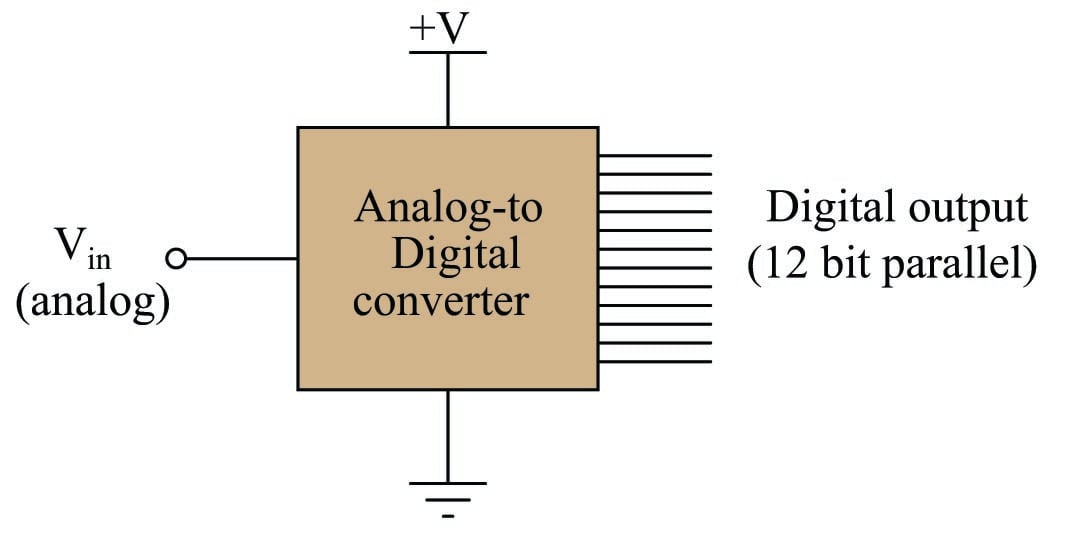
Since the digital data “width” of this ADC is 12 bits, its digital output ranges from 000000000000 to 111111111111, constituting a 12-bit binary integer with a range extending from 000 hexadecimal to FFF hexadecimal, or 0 decimal to 4095 decimal. This integer number is called the count value of the ADC circuit. Although the ADC shown outputs its digital data in parallel form (with separate terminals for the 12 individual bits), many modern ADC chips are designed for serial data output, where a single terminal generates a sequential series of bits timed to the pulse of a clock signal.
Supposing this 12-bit ADC has an analog input voltage range of 0 to 10 volts, how do we relate any given digital number value to a voltage value, or vice-versa? The key here is to understand that the 12-bit resolution of this ADC means it has 212, or 4096 possible count values. The 10 volt DC input range is therefore divided up into 212 - 1, or 4095, discrete increments:
\[\hbox{Analog resolution} = {\hbox{Analog span} \over {2^n - 1}}\]
Where,
\(n\) = Number of binary bits in the output “word”
For our hypothetical 0-10 VDC, 12-bit converter, the analog resolution is 2.442 millivolts. Thus, for any analog signal between 0 mV and 2.442 mV, the ADC’s output should be zero (binary 000000000000); for any analog signal between 2.442 mV and 4.884 mV, the ADC’s output should be one (binary 000000000001); and so on.
As previously mentioned, the digital value output by an ADC is commonly referred to as a count. The word “count” is used in this context as a unit of measurement. For instance, if we subjected our 12-bit ADC to a full-scale input signal of 10 VDC, we would expect to see a full-scale digital output (binary 111111111111) of 4095 “counts.” Since most ADC circuits are designed to be linear, the mathematical relationship between input voltage and digital output “counts” is a simple proportionality:
\[{V_{in} \over V_{full~scale}} = {\hbox{Counts} \over 2^n - 1}\]
We may use this formula to generate a partial table of input and output values for our 0-10 VDC, 12-bit ADC:
| Vin | Counts (decimal) | Counts (hex) |
|---|---|---|
| 0 V | 0 | 000 |
| 2.46 mV | 1 | 001 |
| 3.85 V | 1576 | 628 |
| 4.59 V | 1879 | 757 |
| 6.11 V | 2502 | 9C6 |
| 9.998 V | 4094 | FFE |
| 10 V | 4095 | FFF |
In order to calculate a digital count value from a given input voltage, simply divide that voltage value by the full-scale voltage, then multiply by the full-scale count value and round down to the nearest whole number. For any given voltage value input to the ADC, there is (ideally) one corresponding output “count” value. The converse cannot be said, however: for any given output “count” value, there is actually a range of possible input voltages (the span of that range being the analog resolution of the ADC, in this case 2.442 mV).
To illustrate, let us take one of the table entries as an example: an analog input of 6.11 volts should yield a digital output of (precisely) 2502 counts. However, a digital output of 2502 counts could represent any analog input voltage ranging between 6.10989 volts and 6.11233 volts. This uncertainty is inherent to the process of “digitizing” an analog signal: by using a discrete quantity to represent something infinitely variable, some detail is inevitably lost. This uncertainty is referred to as quantization error: the (potential) error resulting from “quantizing” (digitizing) an inherently analog quantity into a discrete representation.
Quantization error may be reduced (but never eliminated) by using an ADC with greater resolution. A 14-bit ADC operating over the same 0-10 VDC analog input range would have approximately one-quarter the uncertainty of the 12-bit ADC (0.610 mV instead of 2.442 mV). A 16-bit ADC’s uncertainty would only be (approximately) one-sixteenth that of the 12-bit ADC. The number of bits chosen for any particular ADC application is, therefore, a function of how precise the digitization must be.
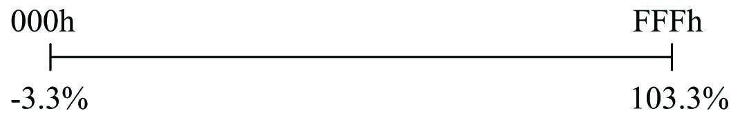
In some data acquisition systems, the digital “count” scale maps to a live-zero analog range. For example, the Siemens model 353 process controller represents process variable, setpoint, and output (“valve”) percentages on a displayed scale of -3.3% to 103.3% with a 12-bit ADC count. For this controller, a digital count of zero (000 hexadecimal) represents an analog signal displayed on the controller’s digital readout of -3.3%, and a full-scale digital count value (FFF hexadecimal) represents a displayed value of 103.3%. We may show the relationship between these two scales in graphical form, like a number line:
At first, the task of translating any analog value into its corresponding digital count value for this scale may seem daunting, but it is really no different than translating an input value into its corresponding output value for any linear instrument. This is something every student of instrumentation learns to do when working with analog-signal instrumentation, where process measurements are represented by 4-20 mA current signals or 3-15 PSI pneumatic pressure signals. If you were given a temperature transmitter with an input range of -100 to 450 degrees Celsius and an output range of 4 to 20 milliamps, and then asked to calculate the appropriate current value corresponding to 300 degrees in that range, the task would be simple. First, you could translate 300 degrees into a per-unit expression of range by subtracting the lower-range value (LRV) of -100 and then dividing by the span (URV \(-\) LRV):
\[{300 - (-100) \over 450 - (-100)} = 0.7273 \hbox{ per unit}\]
After that, you would translate that per-unit figure into a current value:
\[(0.7273)(16) + 4 = 15.636 \hbox{ mA}\]
This general procedure of converting an input value into a per-unit representation of range, then converting that per-unit quantity into an output value, is described in detail in the section beginning on the page. Other methods of performing the same translation between linear input and output ranges.
Converting a digital count value to its respective analog value (or vice-versa) follows the exact same procedure. All we need to do is identify the input and output ranges of the converter circuit, then apply the same formula. One of these ranges will be an analog voltage or current range, while the other will be a count range. If needed, the count value may be translated to or from hexadecimal or binary, because your manual calculations of course would need to be done in decimal format.
For example, suppose one of these Siemens controllers displayed a value of 26.7% on its front panel, and we wished to know what digital (count) value corresponded to this. First, we could translate the panel indication of 26.7% into a per-unit expression of range based on the scale being -3.3% to 103.3%:
\[{{26.7 - (-3.3)} \over {103.3 - (-3.3)}} = {30 \over 106.6} = 0.2814 \hbox{ per unit}\]
Then, we may take this per-unit expression of 0.2814 and multiply it by the span of the known count range (4095 for a 12-bit converter) to arrive at 1152, or 480 hexadecimal (480h).
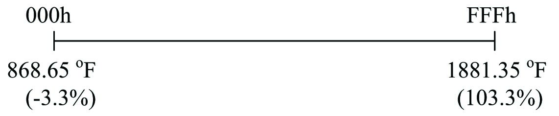
Similarly, if we knew the range of this 12-bit ADC in actual process engineering units, we could translate between ADC counts and the process value by the same method. Suppose we used one of these same controllers to display the temperature of a furnace, where the lower- and upper-range values were 900 deg F and 1850 deg F, respectively. It is important to realize that these lower- and upper-range values represent 0% and 100% of scale, and that the ADC is actually configured to cover a range from -3.3% to 103.3%. In other words, the ADC range “spills over” the specified range of 0 to 100% (900 to 1850 °F) by 3.3% on both ends, equating to 31.35 °F above and below the specified range limits. Thus, the 12-bit ADC’s full-count range of 0 to 4095 (000 to FFF hex) actually covers a temperature range of 868.65 °F to 1881.35 °F:
Suppose we happened to know the ADC count inside this Siemens controller for a certain furnace temperature was A59 hexadecimal (A59h), equal to 2649 in decimal form:
To convert this count value into a temperature, first we convert the count value of 2649 into a per-unit value:
\[{2649 \over 4095} = 0.6469 \hbox{ per unit}\]
Next, we translate this per-unit value into a temperature based on the known LRV and URV range points:
\[(0.6469)(1881.35 - 868.65) + 868.65 = 1523.75 \hbox{ degrees F}\]
Converter Sampling Rate and Aliasing
The next major performance metric for analog signal digitization is how often the analog signal gets converted into digital form. Each time an ADC circuit “samples” its analog input signal, the resulting digital number is fixed until the next sample. This is analogous to monitoring a continuously moving object by taking a series of still photographs. Any changes happening to the analog signal between sampling events are not detected by the converter, and therefore are not represented in the digital data coming from the converter.
It stands to reason, then, that the sampling rate of any ADC must be at least as often as significant changes are expected to take place in the analog measurement. According to the Nyquist Sampling Theorem, the absolute minimum sample rate necessary to capture an analog waveform is twice the waveform’s fundamental frequency. More realistic is to have the ADC sample the waveform ten times or more per cycle.
In general electronics work, for example with the design of electronic test equipment such as digital multimeters (DMMs) and digital storage oscilloscopes (DSOs), sampling rates must be rather fast. Modern digital oscilloscopes may have sampling rates in the billions of samples per second, to allow for the successful digitization of radio-frequency analog signals.
Industrial process measurements are far more forgiving than measurements commonly performed on an electronic technician’s workbench, thankfully. The temperature of a large furnace may be adequately sampled at a rate of only once per minute, if need be. Even “fast” feedback processes such as liquid flow and pressure control may be controlled with reasonable stability by digital systems sampling just a few times per second.
A sampling rate that is too slow (infrequent) may detrimentally affect a measurement or control system in more than one way. First, the time between samples is dead time to the system: time during which the digital system will be completely unresponsive to any changes in process measurement. Excessive dead time in an alarm system means an unnecessary time delay between the alarm event and the alarm signal. Excessive dead time in a feedback control loop leads to oscillation and instability. Another detrimental effect of low sampling rate is something called aliasing: a condition where the digital system “thinks” the frequency of an analog signal is far lower than it actually is.
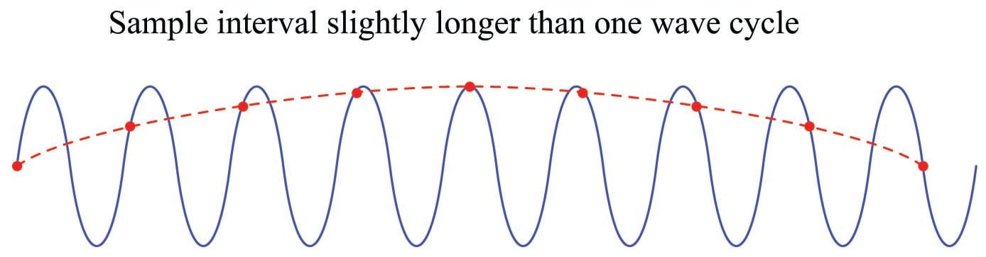
An example of signal aliasing is shown in the following illustration, where a sinusoidal signal (colored blue) is sampled at periods slightly slower than once per cycle (samples marked by red dots). The result (the red, dashed curve) is what appears to be a much lower-frequency signal as seen by the digital system, which only “sees” the values represented by the red dots:
Aliasing can even occur when the sampling rate is slightly faster than the sinusoidal signal’s period, as shown in this illustration:
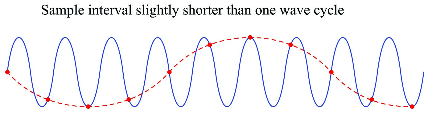
As you can see from these illustrative examples, the troubling nature of aliasing is that it causes the ADC to report a completely incorrect, yet completely plausible signal. The only way to avoid aliasing is to ensure that the sampling rate is much faster than the signal period: a good rule here is to sample at least 10 times per period, for the highest signal frequency of interest.
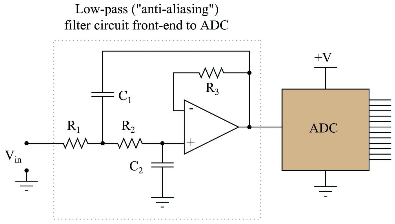
If we cannot set the sampling rate of the ADC to be significantly faster than the highest signal frequency we might encounter, we may avoid aliasing by preventing those high signal frequencies from ever reaching the ADC. This may be done by placing an analog low-pass filter circuit before the ADC’s input. Such a “front-end” circuit is called an anti-aliasing filter:
Aliasing may still occur within digital systems, though, if one portion of a system “samples” the digital output of another portion at too slow of a rate. An example of this might be the rate at which a digital control system (such as a DCS) polls a process variable value collected by a digital sensor network (such as a network of radio-linked process transmitters, or digital fieldbus transmitters). If the DCS polling rate is sufficiently slow compared to the frequency of the signal reported by the digital transmitters, aliasing may result. The best guard against such potential troubles is to synchronize the sampling rates throughout the system, or (alternatively) ensure data sources always output values at a significantly slower rate than any functions reading them. Remember that a practical (minimum) sample rate to signal period ratio is 10:1 to ensure good analog-to-digital conversion integrity.
