 Facebook
 Google
 GitHub
 Linkedin
Digital Representation of Numerical Data
Process measurements are often of an analog nature: the temperature of a furnace, the rate of fluid flow through a pipe, the pressure of a fluid, etc. These data are all analog quantities: infinitely variable, not discrete. Discrete process measurements, such as the number of units passed by on a conveyor belt, are relatively easy to sense and to log in digital form, but analog measurements require special circuitry and methods of numerical representation in order for control systems to manage them.
In order for any digital device to successfully interface with an analog signal, that signal must be digitized by means of an analog-to-digital converter or ADC. In general, ADC circuits receive analog voltage signals from sensors and output binary numbers (count values) proportional to those signals. A typical scale for an ADC is a count of zero (all binary bits = 0) when given a 0 millivolts input, and a full-scale count (all binary bits = 1) when the voltage input value is at its maximum (full-scale). The “full scale” value of an ADC circuit is often a modest DC voltage value of 5 or 10 volts. Details of ADC performance are discussed in a subsequent section of this chapter.
Many of the concerns discussed in this section are relevant to circuits converting digital values into analog signals as well. These digital-to-analog converters, or DACs, are generally used to produce the analog drive signals required of final control elements, like the output of a digital PID controller driving a 4-20 mA analog signal to a control valve positioner.
Integer Number Formats
An integer is any whole number or its negative counterpart (for example, 2, 7, 241, 0, -35, -1022). All modern digital systems represent integer quantities using binary numeration, where integer numbers consist of strings of “bits,” each bit having two possible values: 0 or 1. Unlike the decimal numeration system most people are familiar with where the place-weight values are powers of ten, the place-weight values of binary numeration are powers of two. The following example shows how the integer number six hundred and three is represented in both decimal and binary formats:
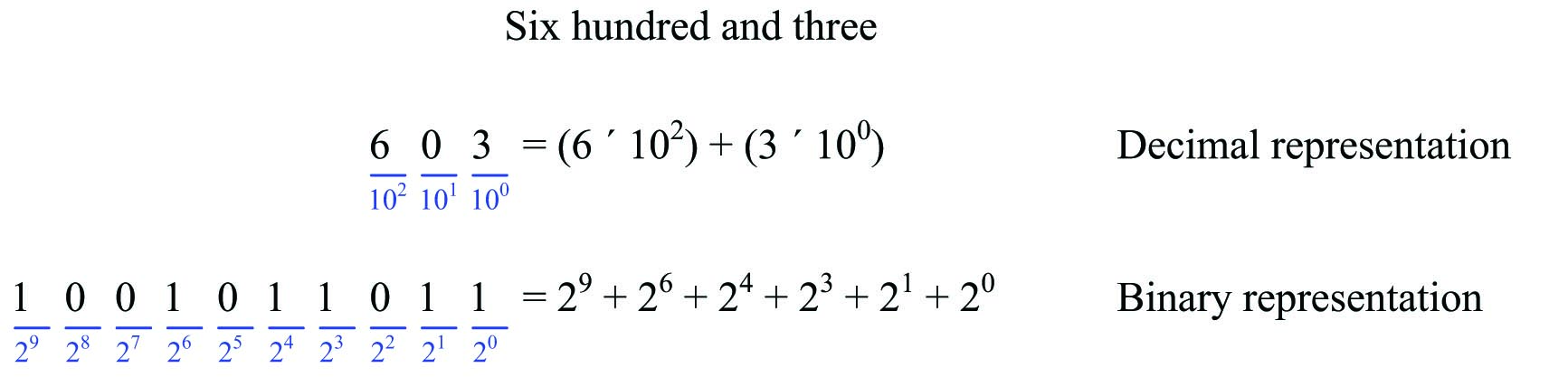
The largest integer value representable in any positive place-weighted format is the base raised to the power of the number of places, minus one. So, for a three-digit decimal number, the largest possible value is 103 - 1 (1000-1 = 999). For a ten-bit binary number, the largest possible value is 210 - 1 (1024-1 = 1023).
The beauty of binary representation is that the individual “bits” are easy to encode in physical form. “1” and “0” values may take the form of voltage levels (“high” or “low”) in an electronic circuit, magnetization states on a magnetic disk or magnetic tape, AC signal frequencies (“high” or “low”) transmitted on a two-conductor cable, pulses of light transmitted through a fiber optic cable, or any other medium capable of representing two different states. This makes binary a natural form of numerical representation for computers.
When representing negative integers, the convention for written numerals is to prepend a “negative” symbol to the left-hand side of the number. In digital machines, this may be emulated by including an extra “sign bit” having a value of either 0 or 1 indicating whether the number is positive or negative. A more common method for negative value representation in digital machines, however, is called two’s complement notation.
Two’s complement notation works by assigning the most significant place-weight a negative weight value. To use a ten-bit binary example showing the number negative three hundred and ninety-six:
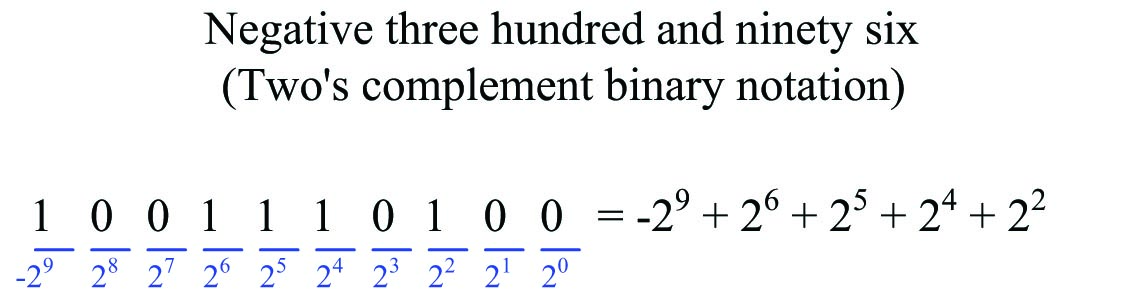
Using this system to represent integer values, the greatest positive number possible is when all bits are “1” with the exception of the most significant bit (MSB). In the case of this ten-bit field, this number would be 0111111111, equaling 29 - 1 or 511. The greatest negative number possible is when the only “1” bit is the MSB. In the case of this ten-bit integer, this number would be 1000000000, equaling -29 or -512. Thus, a ten-bit two’s complement integer may represent values ranging from -512 to +511, inclusive.
Whether binary numbers in a computer use the two’s complement system of notation or not is often the choice of the human being programming the computer. For this reason, it is important to define whether a binary integer used within a computer system to represent data is signed or unsigned. If the integer in question is “signed,” it means the binary number is capable of representing both positive and negative integer values (usually via two’s complement notation). If the integer in question is “unsigned,” it means the binary number is capable only of representing positive values.
For example, an “unsigned” 16-bit integer has a possible numerical value range of 0 to 65535. However, the same 16-bit field – if designated as “signed” using two’s complement place-weighting – has a range of -32768 to +32767.
Digital computers usually organize binary numbers as clusters of bits with a set number of bits. A cluster of eight bits is called a byte. The standard number of bits for most modern computers exceeds one byte, with 16, 32, or even 64 bits’ length being common. Whatever the standard bit-length of a computer’s binary number field may be, it is defined for that computer as a word. Thus, if a digital computer is built to process binary data in 32-bit clusters, one “word” of data within that computer will be 32 bits in length. A “double-word” value for that computer is one where the binary number consists of 64 bits.
Given the typically large bit-lengths of numbers in modern computers, it is conventional to express such quantities in “shorthand” form using hexadecimal numeration. The basic idea of hexadecimal is that every four bits (half of a byte) of a binary number are represented by a single hex character ranging in value from 0 through F (0,1,2,3,4,5,6,7,8,9,A,B,C,D,E,F). For example, the 16-bit binary number 1001001111011110 is equivalent to the four-digit hexadecimal number 93DE:
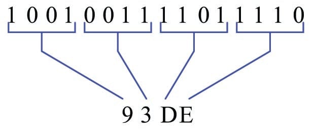
Quite obviously, the hexadecimal number 93DE is a lot easier for human beings to manage than the binary number 1001001111011110. Computer systems providing users with live “views” of numerical values often format those values using hexadecimal numeration, just to simplify the task of interpretation. In conventional programming systems, this long binary number might be written with underscore separators for easier interpretation: 1001_0011_1101_1110.
Fixed-Point Number Formats
The main limitation of integer numbers is their inability to represent quantities between whole numbers such as fractions. For example, a 4-bit integer number may have one of sixteen possible values (zero through fifteen), but it can never represent two-and-a-half.
One solution to this limitation is to re-assign place-weight values to the bits of a binary number, giving some of those bits fractional weights. For example, here is a ten-bit binary number field with a “binary point” separating whole-weighted bits from fractional-weighted bits, representing the quantity 70.375:
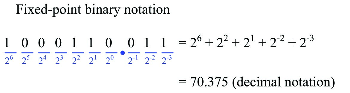
This form of binary notation is referred to as fixed-point, because the “binary point” is fixed in its location. Like any integer variable, this 10-bit binary number consisting of seven whole-weighted bits and three fractional-weighted bits has a definite range of possible values: in this particular case, from 0 to 127.875.
A variation on this theme is to use an integer number whose decimal value is some power-of-ten-times larger than it needs to be, but regard it as though it had a decimal point between two of its digits. I will illustrate this concept by way of anecdote: I once worked on a digital travel-measurement system which displayed the distance a hydraulic ram’s piston traveled using an LED numerical display. The sensor was a pulse encoder providing ten pulses per inch of travel, and this pulse signal directly fed a digital counter circuit which drove the LED display. When the hydraulic ram moved 19.3 inches, the LED display incremented by 193 counts. In order to make this LED display easy to read for human operators, I placed a dab of bright-red fingernail polish on the LED display to make it look as though a decimal point were permanently fixed between the least-significant digit and the next-significant digit. With the fingernail polish dot in place, 193 counts would read as 19.3. A text label saying “inches” was affixed to the right of the LED display, completing the indicator.
This solution is common to many industrial devices. Variable-frequency motor drives (VFDs), for example, often accept speed command values in integer format even though it is often necessary to specify drive frequency down to fractions of a Hertz. In such cases, the VFD manufacturer will program the VFD to imply a decimal point in the received integer number. For instance, if the fixed-point format is specified as XXX.X it means an integer value of 2057 sent to the VFD will be interpreted as 205.7 Hz; a value of 439 will be interpreted as 43.9 Hz; etc.
While fixing a “binary point” in the bit field escapes the limitation of whole-number resolution, a more sophisticated approach known as floating-point representation is a far more flexible way of representing fractional quantities in binary form. This is how most digital computers represent real-world analog quantities in digital form, and is the topic of the next subsection.
Floating-Point Number Formats
Integer numbers, while very commonly used in computers for representing data, are insufficient for tasks requiring the representation of fractional (non-whole) values. Most industrial data points fall into this category, whether it be a temperature measurement (e.g. 428.21 \(^{o}\)C), a gas concentration (e.g. 5.09 ppm of carbon monoxide), a control valve position (e.g. 27.58% open), or a motor speed (e.g. 1592.1 RPM). What we need is a form of binary representation capable of expressing fractional quantities.
One way to do this is to use floating-point number format, where we represent binary quantities using a form resembling scientific notation. Some control systems refer to floating-point numbers as real numbers. Recall how we use scientific notation to represent decimal numbers:
\[1002349 = 1.002349 \times 10^{6}\]
\[678.331 = 6.78331 \times 10^{2}\]
\[0.00004532 = 4.523 \times 10^{-5}\]
The power-of-ten multiplier has the effect of “floating” the decimal point to any position we desire, so that the significant digits of the number may be expressed in “normalized” form (between 1 and 10). This is where the term “floating-point” comes from.
In binary floating-point notation, we use a designated set of bits to represent the significant bits of the number (m), and a second designated set of bits to represent the power-of-two exponent (E):
\[\pm 1.m \times 2^{E}\]
Alert readers will note that the format shown here (±1.m x 2E) provides no way to represent the number zero, since 1.0 x 20 (m = 0 and E = 0) is actually equal to one! Here, floating-point notation must provide special cases of representation. In the IEEE standard, the format shifts to ±0.m x 2E if ever all exponent bits are 0 (E = 0). In order to still be able to represent 1 (1.0 x 20), the IEEE standard assumes the exponent value is biased with a negative number, so that an exponent bit field of 0 does not mean 20, but rather 2-bias. This makes it possible to have an exponent value of 0 using non-zero E bits. Similarly, an exponent field consisting entirely of 1 bits is used as special representation for infinity or for an error code called Not a Number (NaN), depending on the values of the m bits. These special representations are important for handling the results of calculations such as division-by-zero and the square-roots or logarithms of negative numbers.
Given these special cases of representation required in floating-point notation, the task of doing calculations with floating-point numbers requires special processor circuitry designed to implement these rules. Inside a digital computer, this task is managed by a floating-point processor unit, usually a special section of the microprocessor. Some simpler microprocessors cannot support floating-point arithmetic, and thus some control system hardware (usually low-cost PLCs) must do all tasks using integer numbers (or fixed-point notation, if fractional quantities must be represented).
The ANSI/IEEE standard 754-1985 specifies multiple floating-point number formats, including one that is 32 bits in length (“single-precision”) and another that is 64 bits in length (“double-precision”). In the IEEE standard, one bit is reserved for the sign of the number (0 for positive and 1 for negative), a certain number of bits for the power-of-two exponent, and the rest of the bits for the mantissa (the fractional portion of the normalized value). Both formats are shown here:
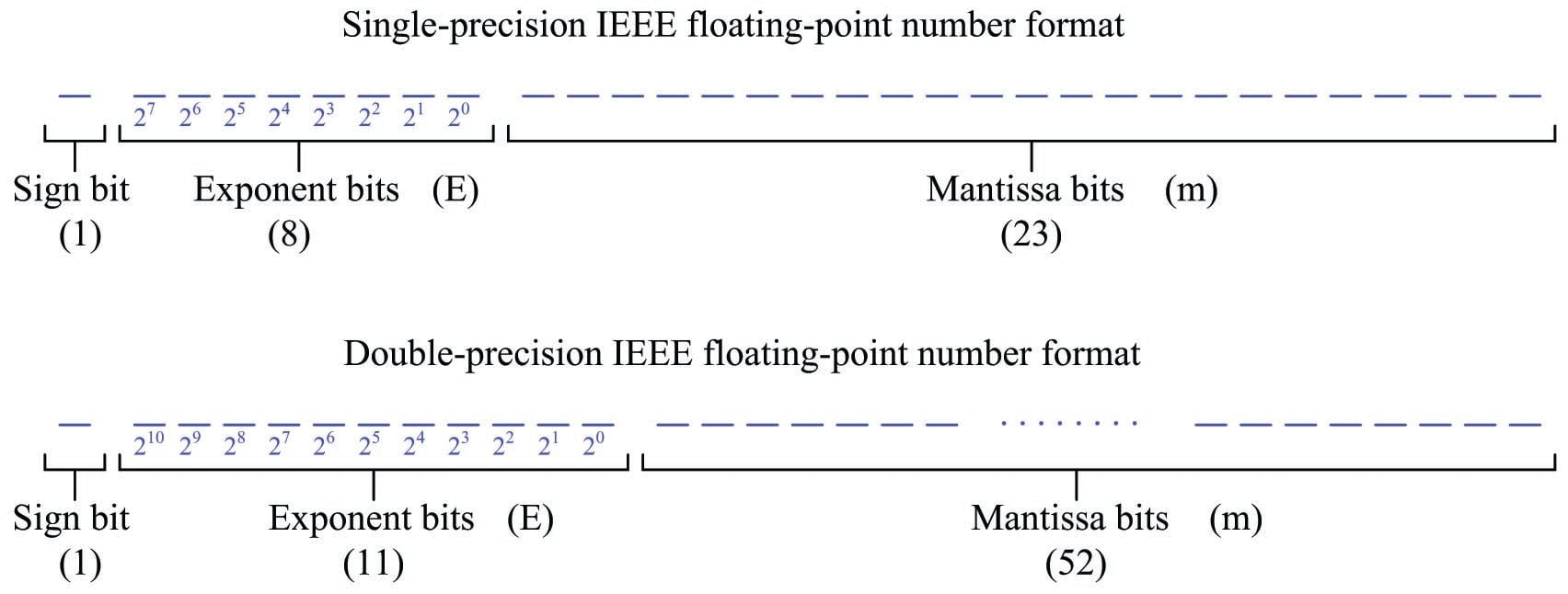
A third floating-point IEEE standard called extended uses 80 total bits: 1 for the sign, 15 for the exponent, and 64 for the mantissa.
Floating-point number representation greatly simplifies the task of digitally calculating real-world values. Integer numbers, by contrast, are rather clumsy when used to represent most real-world measurements or statistics. For this reason, floating-point numbers are sometimes referred to as real values in digital computer systems.
Specific details on IEEE floating-point representation and arithmetic rules extend beyond the scope of this book. For a good primer on the subject, I recommend Michael L. Overton’s excellent paper “Floating Point Representation”.
Example of Industrial Number Formats
To illustrate how different digital data formats are used in industrial systems, we shall explore an example of a human-machine interface (HMI) panel providing graphical view and control of data within a programmable logic controller (PLC). HMI panels are nothing more than special-purpose computers equipped with graphic display screens for displaying data to human operators and pushbuttons (sometimes touch-sensitive graphic screens) for receiving input from human operators.
The following illustration shows how an HMI may be used with a PLC to control electric power to a motor:
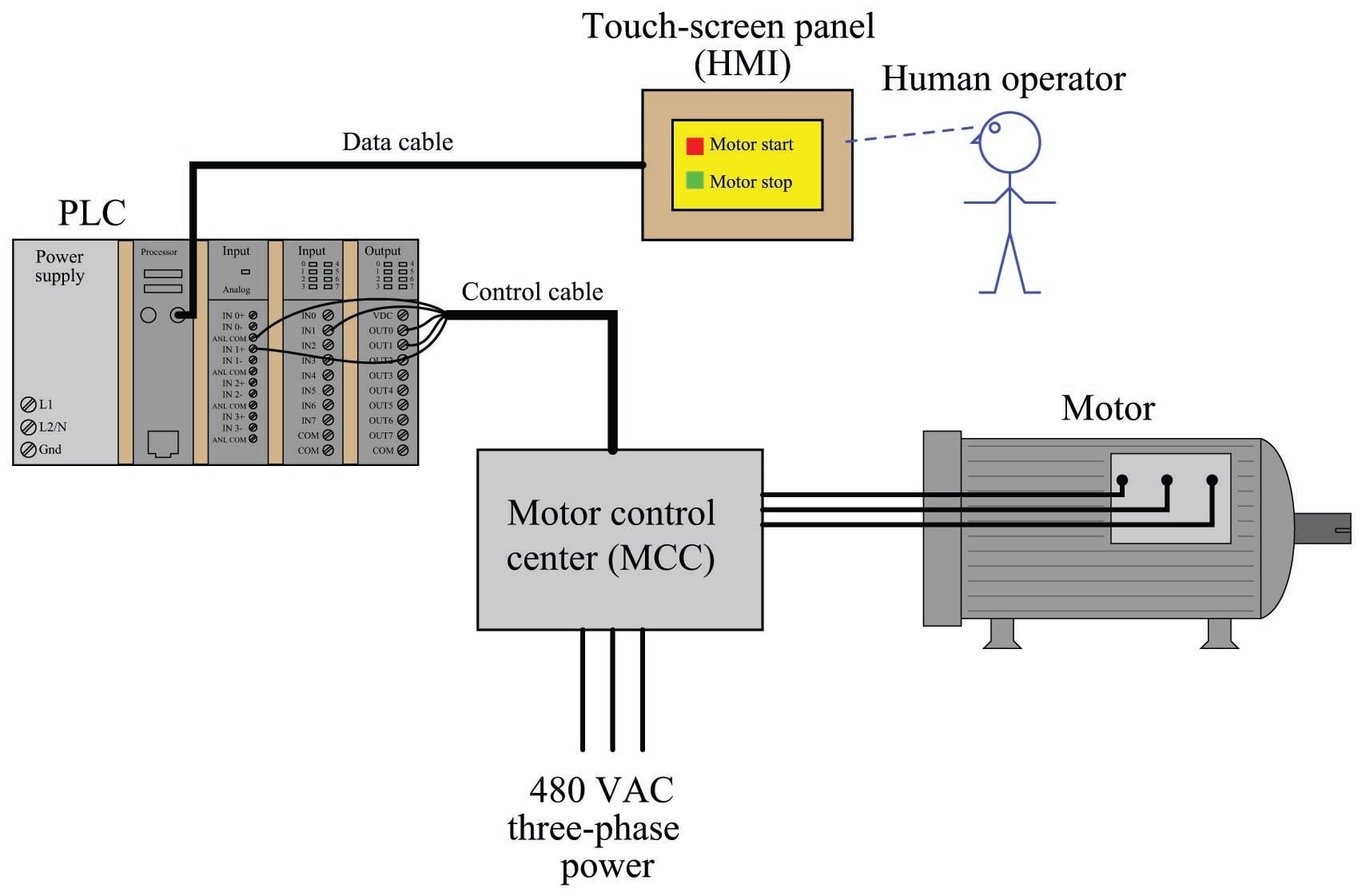
When the operator presses a button on the HMI display to tell the motor to start, the HMI panel sends digital data to the PLC instructing the program within the PLC to activate the motor. The PLC, in turn, receives this data from the HMI and determines whether or not to start the motor. If the motor starts, the PLC sends data back to the HMI confirming the motor’s “run” status, which the HMI indicates to the operator in graphic form.
The configuration software used to set up communication between an HMI panel and the control device typically requires the human programmer (engineer or technician) to specify which data points inside the control device will be accessed by the HMI panel. This is specified in a list called the tag name database. A screen-shot of the tag name database for a particular HMI panel configured to communicate with a PLC using Modbus protocol appears here:
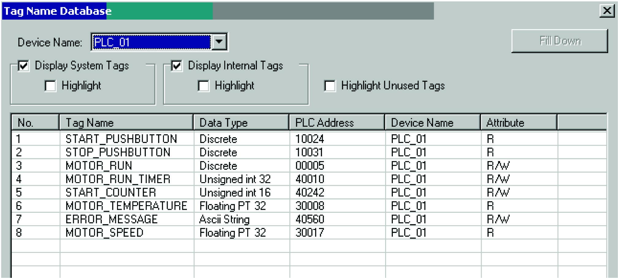
This database table shows the “tag name” assigned to each data point (for easy programming reference), the type of digital data format used, the memory address within the control device (the PLC), the network name of the PLC, and whether the data point is read-only (R), write-only (W), or read/write (R/W) from the perspective of the HMI panel.
Note how the first three tag names are all classified as discrete data. The word “discrete” here is synonymous with Boolean, because it represents single-bit data having only two possible states: on or off, 1 or 0. As the tag names imply, these particular data points are associated with simple on/off states: a pushbutton for starting a motor, another pushbutton for stopping a motor, and a bit representing the motor’s “run” status. Once these tag names, data types, and device address values have been established, the programmer may then link the tags to graphic objects on the screen of the HMI panel. Perhaps a square box with the words “Motor start” may serve to activate the START_PUSHBUTTON bit and cause the PLC to energize the electric motor. An animated graphic image of a motor may be programmed to show rotation if the MOTOR_RUN bit is set, and show no motion if that same bit is cleared.
Four other data types appear in this tag name database, each one representing different forms of information:
- Unsigned 16-bit integer
- Unsigned 32-bit integer
- Floating-point 32-bit (also known as “Real” number format)
- ASCII string
Two “unsigned integer” data points represent motor run time and a “start counter” for keeping count of how many times the motor has been started. The timer is a 32-bit integer value, while the counter is a 16-bit integer value. Being unsigned integers (no two’s complement notation), the numerical range of the timer is 0 to 4,294,967,295 (232 - 1) and the numerical range of the counter is 0 to 65535 (216 - 1). The large range afforded by the timer’s 32-bit word length allows up to 136.2 years’ worth of recorded continuous motor run time, assuming a timer resolution of one second per count.
Two of these data points use 32-bit floating-point format to represent analog motor data: motor temperature and motor speed. Given the units of measurement common to these types of variables (degrees Celsius or Fahrenheit, revolutions per minute), a resolution of ±1 as given by an integer number would probably be insufficient for the task. Instead, the operator should be able to read fractions of a degree in temperature, and fractions of an RPM motor speed. This necessity to display numerical values with resolution less than 1 unit dictates the use of the floating-point data type.
The last data type represented in this tag name database is an “ASCII string,” which means a series of bytes (8-bit groupings) representing text data, such as a message. In this particular case, the tag name itself betrays the purpose of the data: ERROR_MESSAGE. The PLC obviously has the ability to generate text messages and send them to the HMI panel to communicate specific errors to the operator.

I clearly understand now the evolution of digital technology and its impact on automating and communicating different process variables.
I now clearly understand the evolution of digital technology and its impact on data transfers and resolving communication bottleneck easing devices communications .