Facebook
 Google
 GitHub
 Linkedin
Feedforward with Dynamic Compensation
As we have seen, feedforward control is a way to improve the stability of a feedback control system in the face of changing loads. Rather than rely on feedback to make corrective changes to a process only after some load change has driven the process variable away from setpoint, feedforward systems monitor the relevant load(s) and use that information to preemptively make stabilizing changes to the final control element such that the process variable will not be affected. In this way, the feedback loop’s role is to merely “trim” the process for factors lying outside the realm of the feedforward system.
At least, this is how feedforward control is supposed to work. One way feedforward controls commonly fail to live up to their promise is if the effects of load changes and of manipulated variable changes possess different time lags in their respective effects on the process variable. This is a problem in feedforward control systems because it means the corrective action called for in response to a change in load will not affect the process variable at the same time, or in the same way over time, as the load will. In order to correct this problem, we must intelligently insert time lags (or advancing time-based functions called leads) into the control system to equalize the time lags of load and feedforward correction. This is called dynamic compensation.
The following subsections will explore illustrative examples to make both the problem and the solution(s) clear.
A common area of confusion among students first approaching this topic is deciding where to place the dynamic compensation function in a feedforward control system. The answer to this question is surprisingly simple, although it may seem elusive at first glance. The key is found in the following principle: the only time-dynamic we have the ability to alter with our control system is the dynamic of the final control element. We cannot alter the time-dynamic of the load’s effect on the process variable, as that is strictly a function of process physics. Therefore, when we test a process employing feedforward control with an eye toward incorporating dynamic compensation, we must measure the time lag of the load’s effect on PV and also the time lag of our final control element’s effect on PV, then compare those two time lags. If the final control element’s time lag is shorter (quicker) than the load’s, then we must add a delay or lag to the feedforward signal so that the final control element’s preemptive action does not occur too soon. If the final control element’s time lag is longer (slower) than the load’s, then we must either find a way to alter the process itself to decrease the load’s time lag, or add a “lead” function to the feedforward signal in order to advance the final control element’s response and thereby ensure the preemptive action does not occur too late. Remember, all we can do with dynamic compensation is alter how the final control element responds (i.e. how slowly or quickly the preemptive action of feedforward occurs). The load’s effect on the process variable is fixed by the physics of the process and therefore lies beyond our direct control.
Dead time compensation
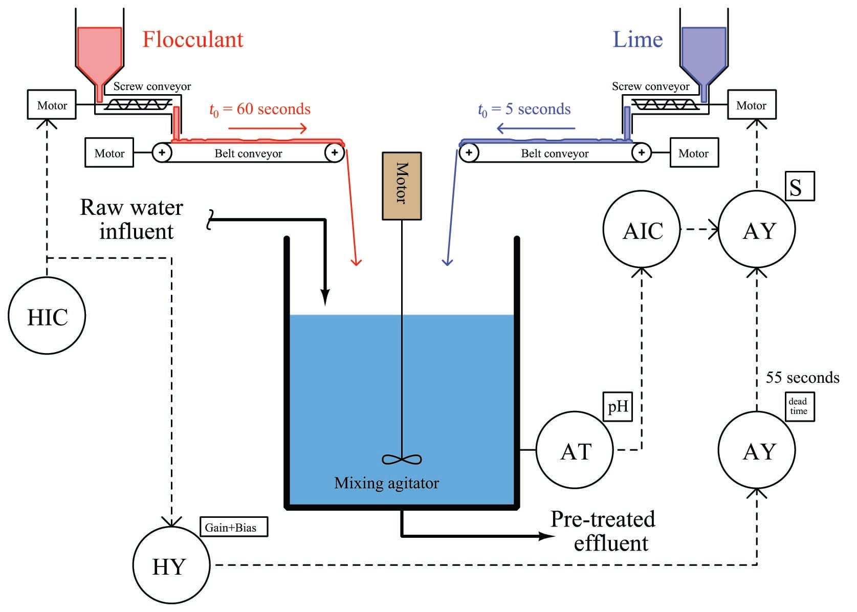
Examine the following control system P&ID showing the addition of flocculant (a chemical compound used in water treatment to help suspended solids clump together for easier removal by filtering and/or gravity clarification) and lime for pH balance. Flocculant is necessary to expedite the removal of impurities from the water, but some flocculation compounds have the unfortunate effect of decreasing the pH value of the water (turning it more acidic). If the water’s pH value is too low, the flocculant ironically loses its ability to function. Thus, lime (an alkaline substance – high pH value) must be added to the water to counter-act the flocculant’s effect on pH to ensure efficient flocculation. Both substances are powders in this water pre-treatment system, metered by variable-speed screw conveyors and carried to the mixing tank by belt-style conveyors:
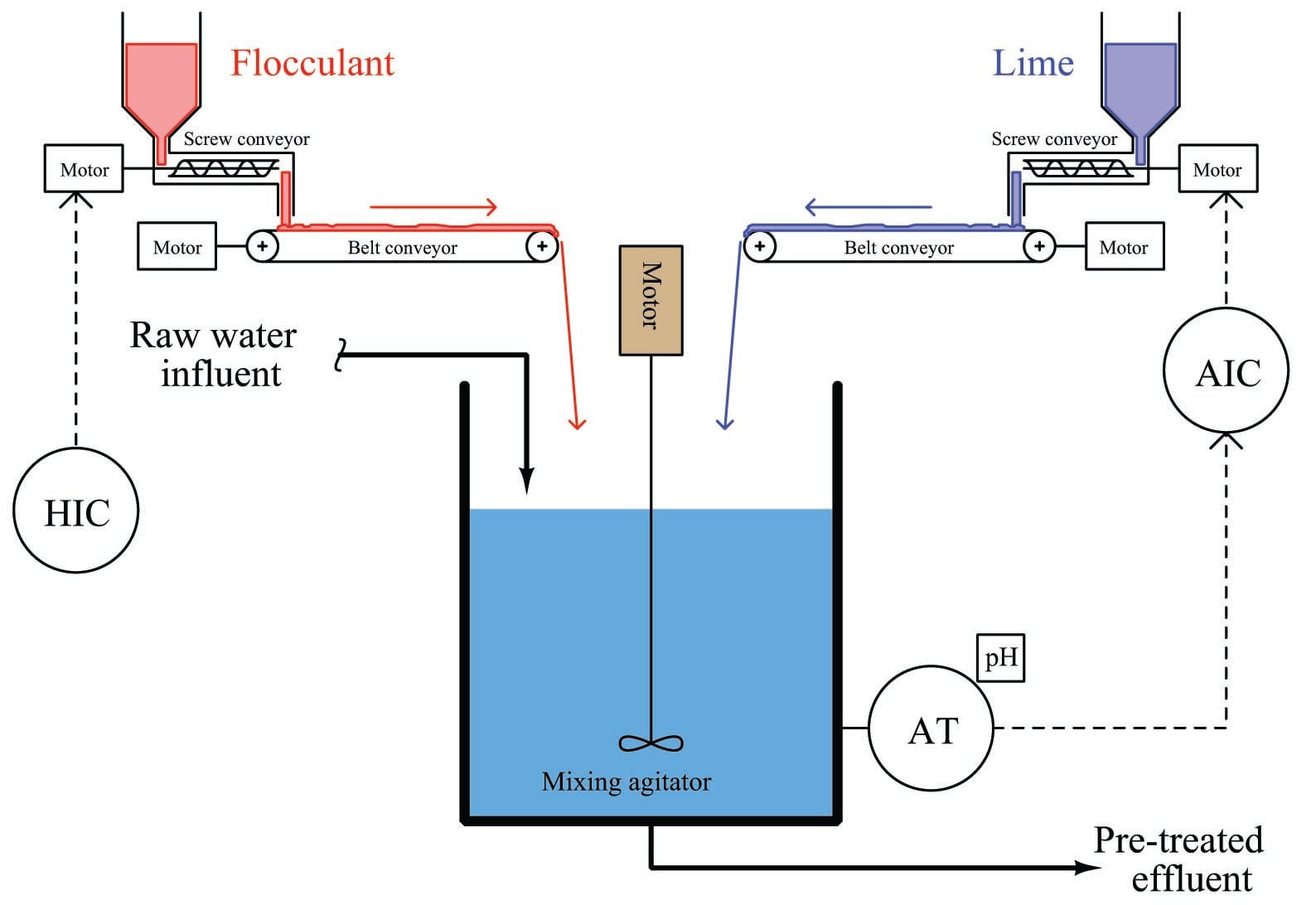
The control system shown in this P&ID consists of a pH analyzer (AT) transmitting a signal to a pH indicating controller (AIC), adjusting the speed of the lime screw conveyor. The flocculant screw conveyor speed is manually set by a hand indicating controller (HIC) – sometimes known as a manual loading station – adjusted when necessary by experienced water treatment operators who periodically monitor the effectiveness of flocculation in the system.
This simple feedback control system will work fine in steady-state conditions, but if the operator suddenly changes flocculant flow rate into the mixing vessel, there will be a temporary deviation of pH from setpoint before the pH controller is able to find the correct lime flow rate into the vessel to compensate for the change in flocculant flow. In other words, flocculant feed rate into the mixing tank is a load for which the pH control loop must compensate.
Dynamic response could be greatly improved with the addition of feedforward control to this system:
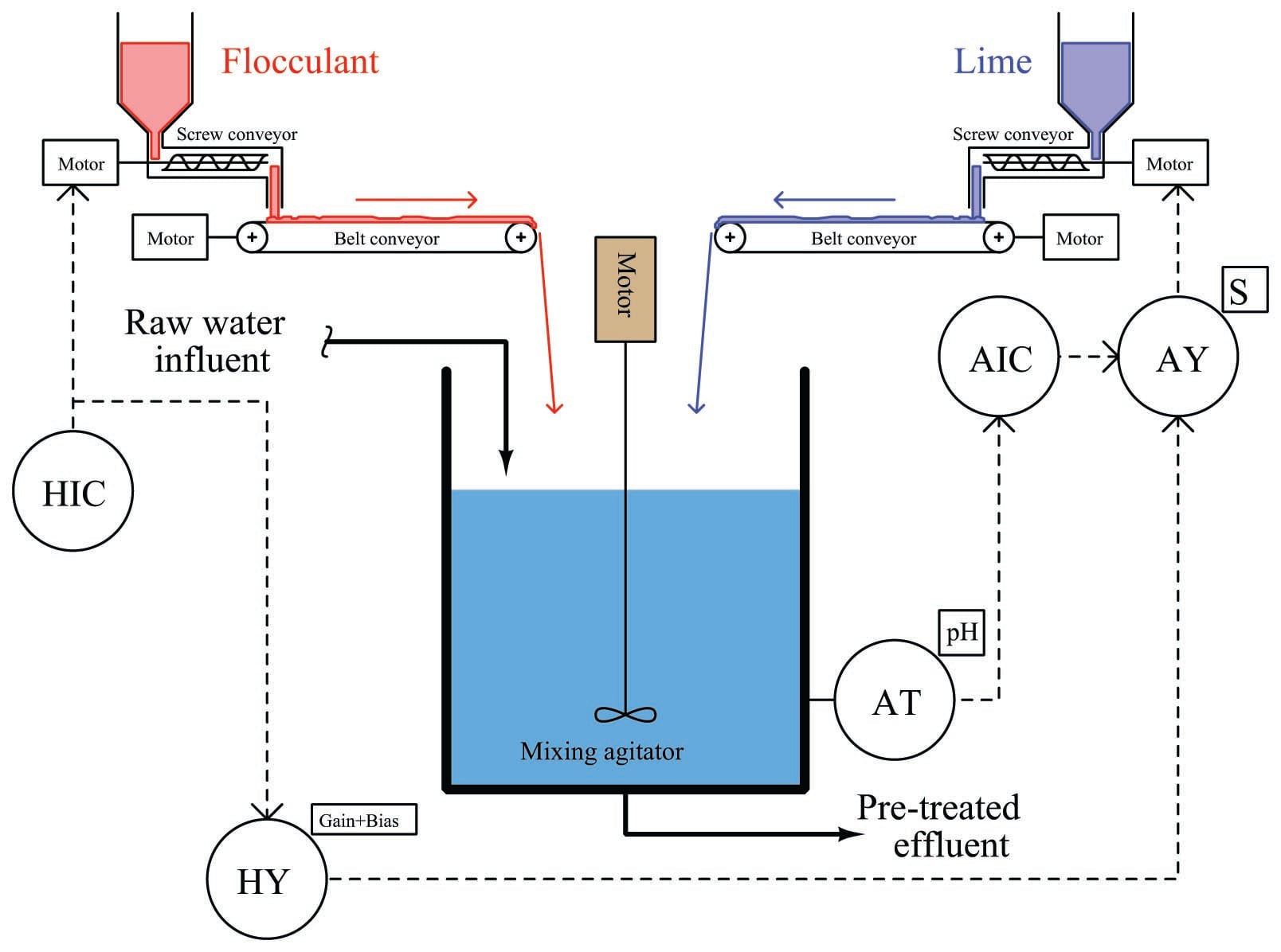
Here, the hand controller’s signal gets added to the pH controller’s output signal to directly influence lime feed rate in addition to acting as a control signal to the flocculant screw conveyor motor drive. If an operator changes the flocculant feed rate, the lime feed rate will immediately adjust to compensate, before any change in pH value takes place in the water. Ideally, the pH controller need only make minor “trim” adjustments to lime feed rate, while the feedforward signal does most of the work in maintaining a steady pH value. The proper proportioning and offset between flocculant and lime feed rates is established in the gain/bias function, which is “tuned”1010 to ensure the feedforward signal does not over- or under-react, calling for too much (or too little) lime to compensate.
Even if all components in the feedforward system have been calibrated and configured properly, however, a potential problem still lurks in this system which can cause the pH value to temporarily deviate from setpoint following flocculant feed rate changes. This problem is the transport delay – otherwise known as dead time – inherent to the two belt conveyors transporting both flocculant and lime powder from their respective screw conveyors to the mixing vessel. If the rotational speed of a screw conveyor changes, the flow rate of powder exiting that screw conveyor will immediately and proportionately change. However, the belt conveyor imposes a time delay before the new powder feed rate enters the mixing vessel. In other words, the water in the vessel will not “see” the effects of a change in flocculant or lime feed rate until after the belt conveyor’s time delay has elapsed. This is not a problem if the dead times of both belt conveyors are exactly equal, since this means any compensatory change in lime feed rate initiated by the feedforward system will reach the water at exactly the same time the new flocculant rate reaches the water. So long as flocculant and lime feed rates are precisely balanced with one another at the point in time they reach the mixing vessel, pH should remain stable. But what if their arrival times are not coordinated – what will happen to pH then?
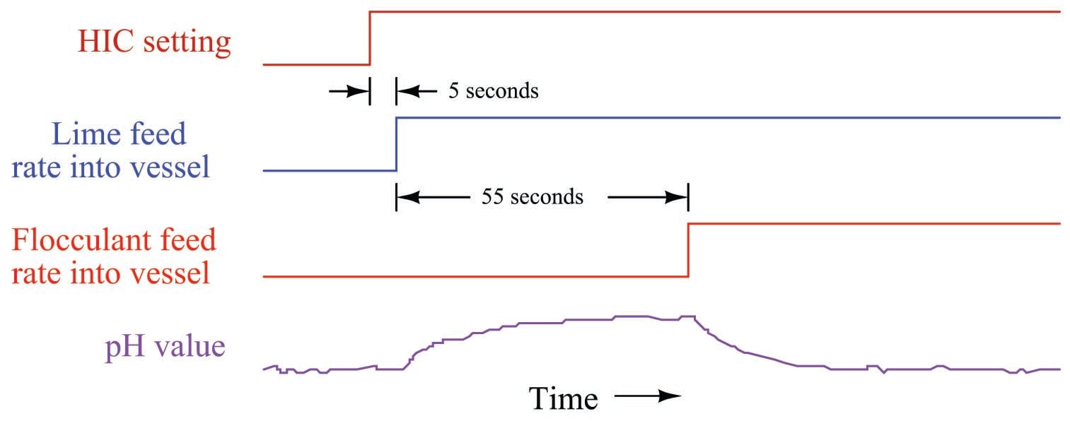
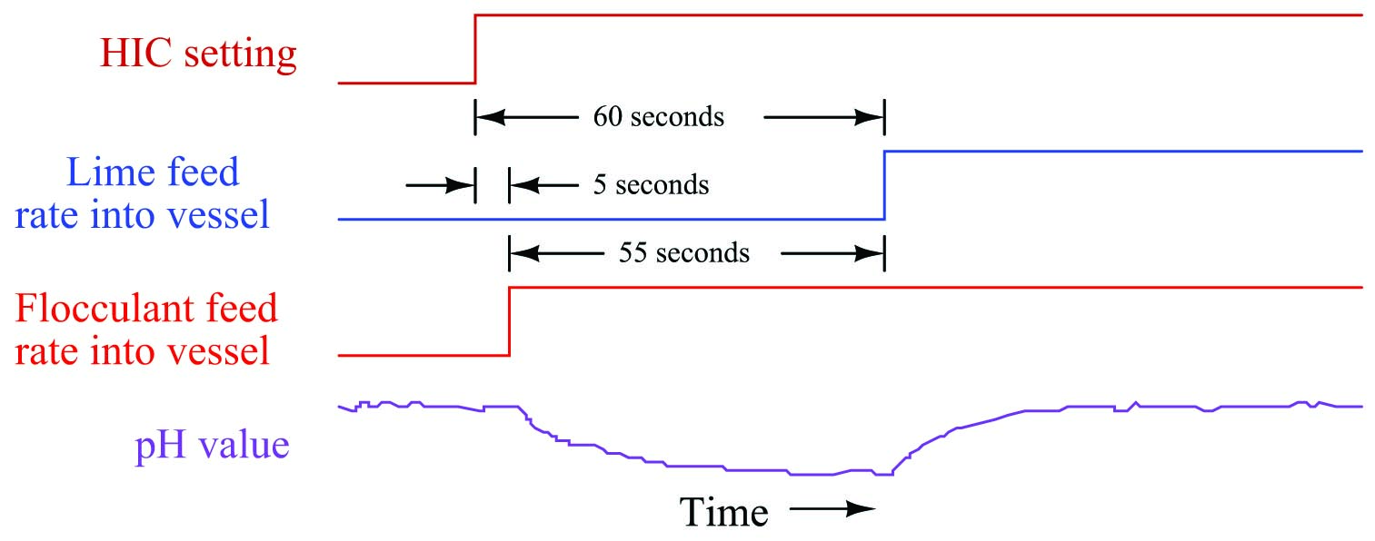
Let us engage in a “thought experiment” to explore the consequences of the flocculant conveyor belt moving much slower than, and/or being much longer than, the lime conveyor belt. Suppose the flocculant belt imposed a dead time of 60 seconds on flocculant powder making it to the vessel, while the lime belt only delayed lime powder transit by 5 seconds from screw conveyor to mixing tank. This would mean changes in flocculant flow (set by the hand controller) would compensate with changes in lime flow 55 seconds too soon. Now imagine the human operator making a sudden increase to the flocculant powder feed rate. The lime feed rate would immediately increase thanks to the efforts of the feedforward system. However, since the increased flow rate of lime powder will reach the mixing vessel 55 seconds before the increased flow rate of flocculant powder, the effect will be a temporary increase in pH value beginning about 5 seconds after the operator’s change, and then a settling of pH value back to setpoint1011, as shown in this timing diagram:
The obvious solution to this problem is to mechanically alter the belt conveyor systems for equal transport times of flocculant and lime powders. If this is impractical, we may achieve a similar result by incorporating another signal relay (or digital function block) inserting dead time into the feedforward control system. In other words, we can modify the control system in such a way to emulate what would be impractical to modify in the process itself.
This new function will add a dead time of 55 seconds to the feedforward signal before it enters the summer, thus delaying the lime feed rate’s response to feedforward effect by just the right amount of time such that any lime feed rate changes called for by feedforward action will arrive at the vessel simultaneously with the changed flocculant feed rate:
Adding time-based functions to a control system in order to equalize inherently unequal time delays in the physical process is called dynamic compensation. It is important to note that dynamic compensation cannot make physically unequal time lags equal – all it does is modify the feedforward system so that signal’s effect arrives at the right time to compensate the load. In simple terms, we can only use dynamic compensation to modify the FCE’s behavior, not the process behavior. Here, there is absolutely nothing the feedforward system can do to speed up the slower flocculant belt, so instead we chose to slow down the feedforward manipulation of lime flow to make it match the flocculant flow.
Note how the feedback pH controller’s loop was purposely spared the effects of the added dead time function, by placing the function outside of that controller’s feedback loop. This is important, as dead time in any form is the bane of feedback control. The more dead time within a feedback loop, the easier that loop will tend to oscillate. By strategically placing the dead time function before the summing relay rather than after (between the summer and the lime screw conveyor motor drive), the feedback control system still achieves minimum response time while only the feedforward signal gets delayed.
Let us now consider the same flocculant and lime powder control system, this time with transport delays reversed between the two belt conveyors. If the flocculant conveyor belt is now the fast one (5 seconds dead time) and the lime belt slow (60 seconds), the effects of flocculant feed rate changes will be reversed. An increase in flocculant powder feed rate to the vessel will result in a drop in pH beginning 5 seconds after the HIC setting change, followed by a rise in pH value after the additional lime feed rate finally reaches the vessel:
What is happening here is that the feedforward signal’s effect is coming too late. In a perfect world our lime flow rate into the mixing vessel should change at the same time that the flocculant flow rate changes. Instead, our lime flow rate’s necessary increase happens 55 seconds too late to prevent the pH from deviating.
It would be possible to compensate for the difference in conveyor belt transport times using a special relay in the same location of the feedforward signal path as before, if only there was such a thing as a relay that could predict the future exactly 55 seconds in advance!1012. Since no such device exists (or ever will exist), we must apply dynamic compensation elsewhere in the feedforward control system.
If a time delay is the only type of compensation function at our disposal, then the only thing we can delay in this system to make the two dead times equal is the flocculation feed rate. Thus, we should place a 55-second dead time relay in the signal path between the hand indicating controller (HIC) and the flocculant screw conveyor motor drive.
This diagram shows the proper placement of the dead time function:
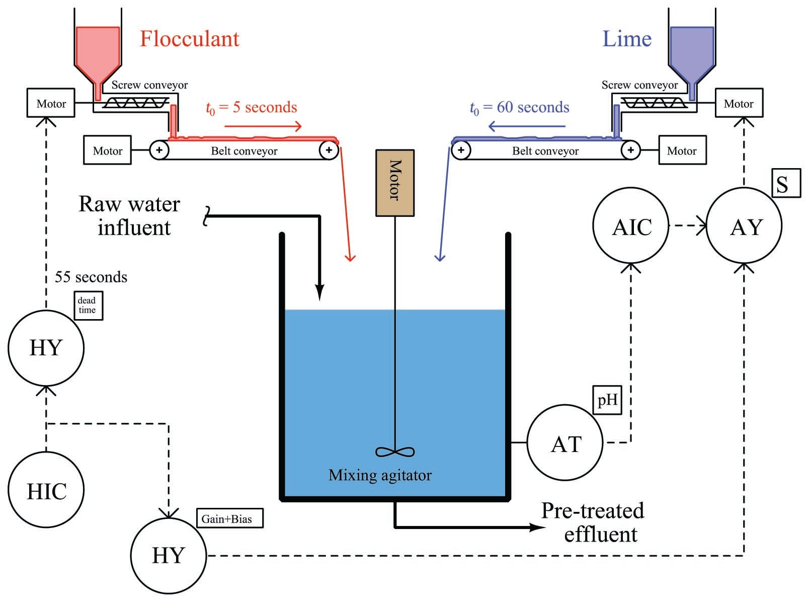
With this dead time relay in place, any change in flocculation feed rate initiated by a human operator will immediately adjust the feed rate of lime powder, but delay an adjustment to flocculant powder feed rate by 55 seconds, so the two powders’ feed rate changes arrive at the mixing vessel simultaneously.
Bear in mind that this solution will really only work in a system like this where the major load happens to be controlled by the human operator. In most processes the load variable is not under anyone’s control, making it difficult if not impossible to purposely delay its action. If the load has a shorter dead time than the compensation, there is usually little we can do within the control strategy to equalize those effects for better dynamic stability. Typically, the best solution is to physically alter the process (e.g. slow down the flocculant belt conveyor’s speed) so that the load and compensation dead times are closer to being equal.
Lag time compensation
Process time delays characterized by pure transport delay (dead time) are less common in industry than other forms of time delays, most notably lag times1013. A simple “lag” time is the characteristic exhibited by a low-pass RC filter circuit, where a step-change in input voltage results in an output voltage asymptotically rising to the new voltage value over time:
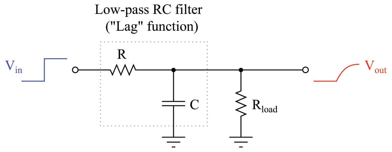
The time constant (\(\tau\)) of such a system – be it an RC circuit or some other physical process – is the time required for the output to move 63.2% of the way to its final value (\(1 - e^{-1}\)). For an RC circuit such as the one shown, \(\tau = RC\) (assuming \(R_{load} >> R\) so the load resistance will have negligible effect on timing).
Lag times differ fundamentally from dead times. With a dead time, the effect is simply time-delayed by a finite amount from the cause, like an echo. With a lag time, the effect begins at the exact same time as the cause, but does not follow the same rapid change over time as the cause. Like dead times in a feedforward system, it is quite possible (and in fact usually the case) for loads and final control variables to have differing lag times regarding their respective effects on the process variable. This presents another form of the same problem we saw in the two-conveyor water pre-treatment system, where an attempt at feedforward control was not completely successful because the corrective feedforward action did not occur with the same amount of time delay as the load.
To illustrate, we will analyze a heat exchanger used to pre-heat fuel oil before being sent to a combustion furnace. Hot steam is the heating fluid used to pre-heat the oil in the heat exchanger. As steam gives up its thermal energy to the oil through the walls of the heat exchanger tubes, it undergoes a phase change to liquid form (water), where it exits the shell of the exchanger as “condensate” ready to be re-boiled back into steam.
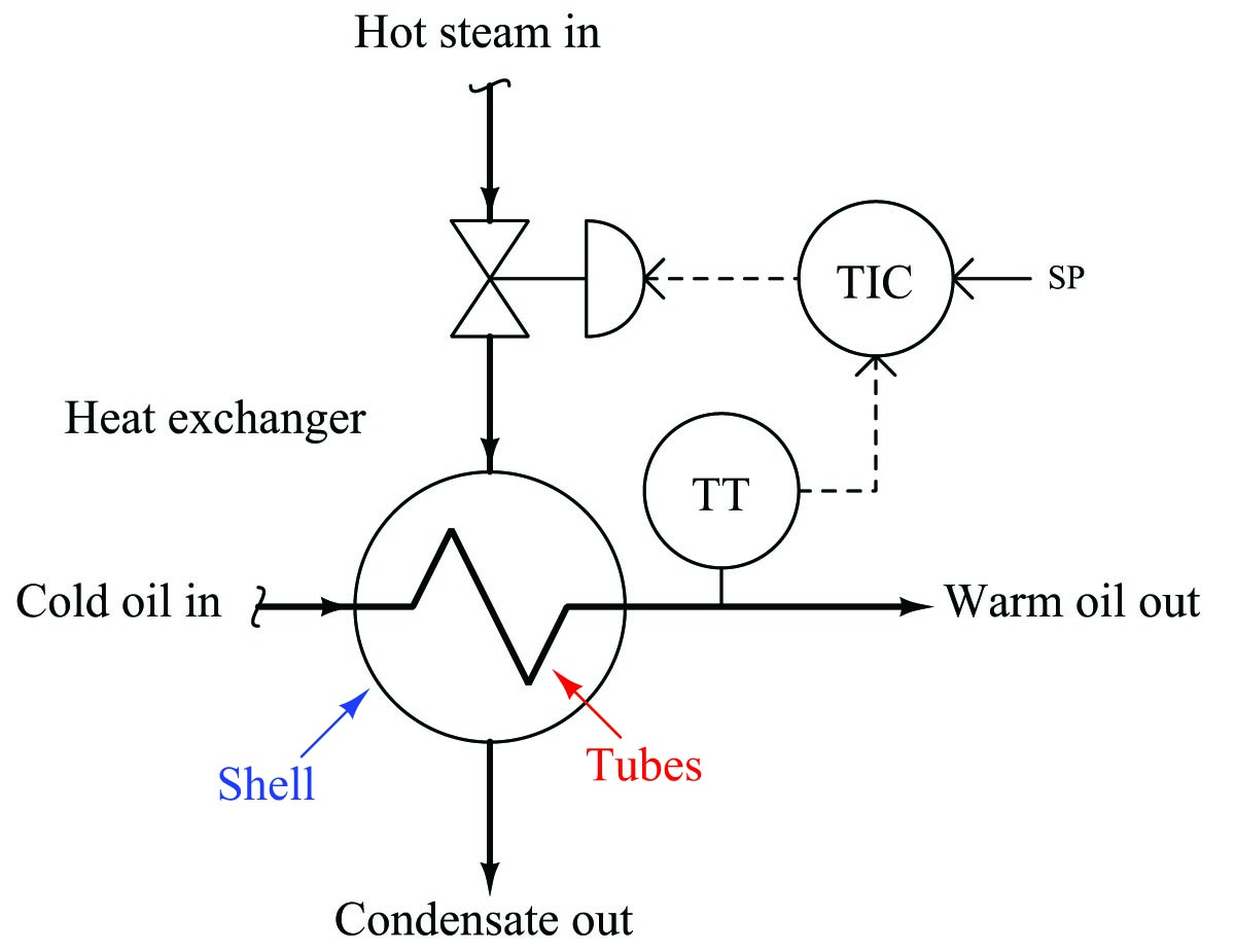
A simple feedback control system regulates steam flow to the heat exchanger, maintaining the discharge temperature of the oil at a constant setpoint value:
Once again, it should come as no surprise to us that the outlet temperature will suffer temporary deviations from setpoint if load conditions happen to change. The feedback control system may be able to eventually bring the exiting oil’s temperature back to setpoint, but it cannot begin corrective action until after a load has driven the oil temperature off setpoint. What we need for improved control is feedforward action in addition to feedback action. This way, the control system can take corrective action in response to load changes before the process variable gets affected.
Suppose we know that the dominant load in this system is oil flow rate1014, caused by changes in demand at the combustion furnace where this oil is being used as fuel. Adapting this control system to include feedforward is as simple as installing an oil flow transmitter, a gain/bias function, and a summing function block:
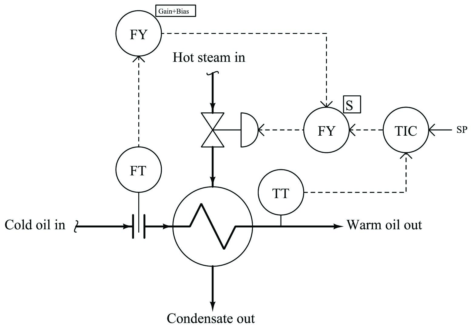
With feedforward control action in place, the steam flow rate will immediately change with oil flow rate, preemptively compensating for the increased or decreased heat demand of the oil. In other words, the feedforward system attempts to maintain energy balance in the process, with the goal of stabilizing the outlet temperature:
There is a problem of time delay in this system, however: a change in oil flow rate has a faster effect on outlet temperature than a proportional change in steam flow rate. This is due to the relative masses impacting the temperature of each fluid. The oil’s temperature is primarily coupled to the temperature of the tubes, whereas the steam’s temperature is coupled to both the tubes and the shell of the heat exchanger. So, the steam has a greater mass to heat than the oil has to cool, giving the steam a larger thermal time constant than the oil.
For the sake of illustration, we will assume transport delays are short enough to ignore1015, so we are only dealing with different lag times between the oil flow’s effect on temperature and the steam flow’s effect on temperature.
This is what would happen to the heated oil temperature if steam flow were held constant and oil flow were suddenly increased:
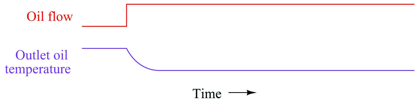
Increased oil flow convects heat away from the steam at a faster rate than before, resulting in decreased oil temperature. This drop in temperature is fairly quick, and is self-regulating.
By contrast, this is what would happen to the heated oil temperature if oil flow were held constant and steam flow were suddenly increased:
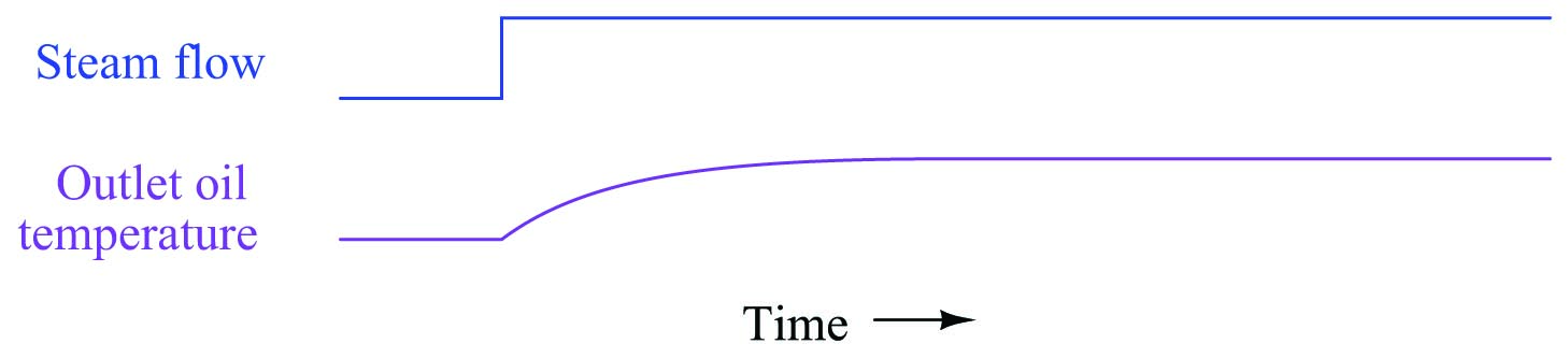
Increased steam flow convects heat into the oil at a faster rate than before, resulting in increased oil temperature. This rise in temperature is also self-regulating, but much slower than the temperature change resulting from a proportional adjustment in oil flow. In other words, the time constant (\(\tau\)) of the process with regard to steam flow changes is greater than the time constant of the process with regard to oil flow changes (\(\tau_{steam} > \tau_{oil}\)).
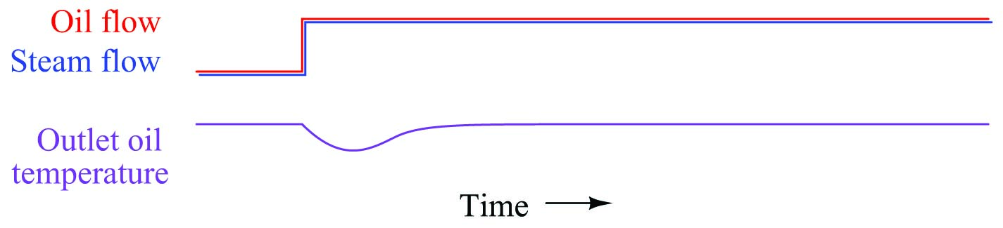
If we superimpose these two effects, as will be the case when the feedforward system is working (without the benefit of feedback “trim” control), what we will see when oil flow suddenly increases is a “fight” between the cooling effect of the increased oil flow and the heating effect of the increased steam flow. However, it will not be a fair fight: the oil flow’s effect will temporarily win over the steam’s effect because of the oil’s faster time constant. Another way of stating this is to say the feedforward action temporarily under-compensates for the change in load. The result will be a momentary dip in outlet temperature before the system achieves equilibrium again:
The solution to this problem is not unlike the solution we applied to the water treatment system: we must somehow equalize these two lag times so their superimposed effects will directly cancel, resulting in an undisturbed process variable. An approximate solution for equalizing two different lag times is to cascade two lags together in order to emulate one larger lag time1016. This may be done by inserting a lag time relay or function block in the feedforward system.
When we look at our P&ID, though, a problem is immediately evident. The lag time we need to slow down is the lag time of the oil flow’s effect on temperature. In this system, oil flow is a wild variable, not something we have the ability to control (or delay at will). Our feedforward control system can only manipulate the steam valve position in response to oil flow, not influence oil flow in order to give the steam time to “catch up.”
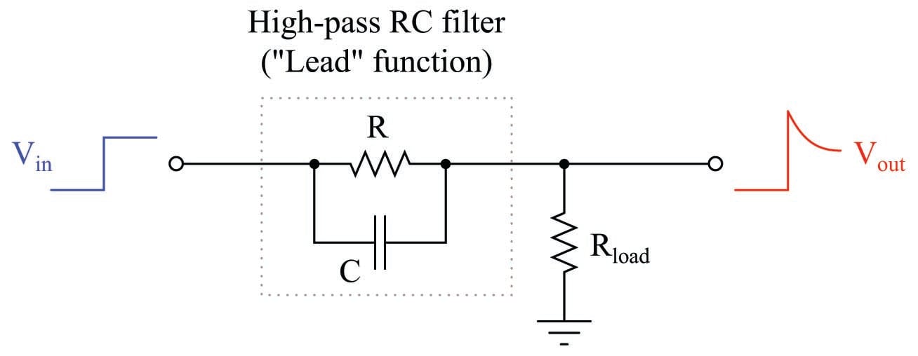
If we cannot slow down the time constant inherent to the wild variable (oil flow), then the best we can do is speed up the time constant of the variable we do have influence over (steam flow). The solution is to insert something called a lead function into the feedforward signal driving the steam valve. A “lead” is the mathematical inverse of a lag. If a lag is modeled by an RC low-pass filter circuit, then a “lead” is modeled by an RC high-pass filter circuit:
Being mathematical inverses of each other, a lead function should perfectly cancel a lag function when the output of one is fed to the input of the other, and when the time constants of each are equal. If the time constants of lead and lag are not equal, their cascaded effect will be a partial cancellation. In our heat exchanger control application, this is what we need to do: partially cancel the steam valve’s slow time constant so it will be more equal with the oil flow’s time constant. Therefore, we need to insert a lead function into the feedforward signal path.
A lead function will take the form of either a physical signal relay or (more likely with modern technology) a function block executed inside a digital control system. The proper place for the lead function is between the oil flow transmitter and the summation function:
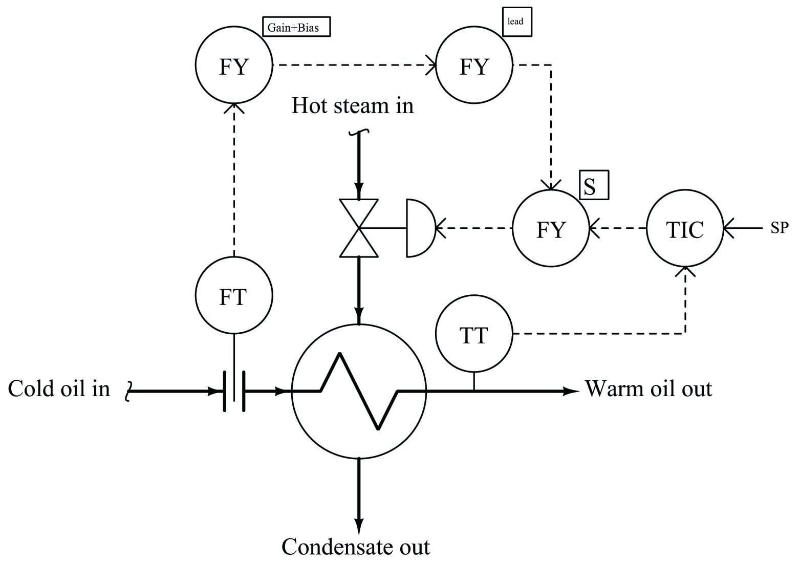
Now, when the oil flow rate to this heat exchanger suddenly increases, the lead function will add a “surge” to the feedforward signal before it goes to the summing function, quickly opening the steam valve further than usual and sending a surge of steam to the exchanger to help overcome the naturally sluggish response of the oil temperature to changes in steam flow. The feedforward action won’t be perfect with this lead function added, but it will be substantially better than if there was no dynamic compensation added to the feedforward signal.
Lead/Lag and dead time function blocks
The addition of dynamic compensation in a feedforward control system may require a lag function, a lead function, and/or a dead time function, depending on the nature of the time delay differences between the relevant process load and the system’s corrective action. Modern control systems provide all these functions as digital function blocks. In the past, these functions could only be implemented in the form of individual instruments with these time characteristics, called relays. As we have already seen, lead and lag functions may be rather easily implemented as simple RC filter circuits. Pneumatic equivalents also exist, which were the only practical solution in the days of pneumatic transmitters and controllers. Dead time is notoriously difficult to emulate using analog components of any kind, and so it was common to use lag-time elements (sometimes more than one connected in series) to provide an approximation of dead time.
With digital computer technology, all these dynamic compensation functions are easy to implement and readily available in a control system. Some single-loop controllers even have these capabilities programmed within, ready to use when needed.
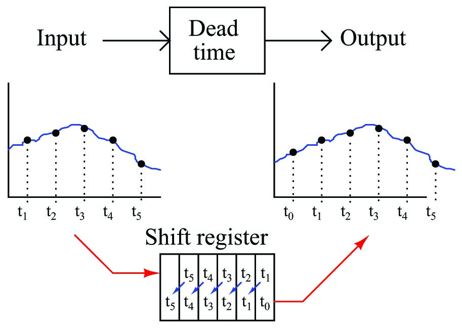
A dead time function block is most easily implemented using the concept of a first-in, first-out shift register, sometimes called a FIFO. With this concept, successive values of the input variable are stored in a series of registers (memory), their progression to the output delayed by a certain amount of time:
Lead and lag functions are also implemented digitally in modern controllers and control systems, but they are actually easier to comprehend in their analog (RC circuit) forms. The most common way lead and lag functions are found in modern control systems is in combination as the so-called lead/lag function, merging both lead and lag characteristics in a single function block (or relay):
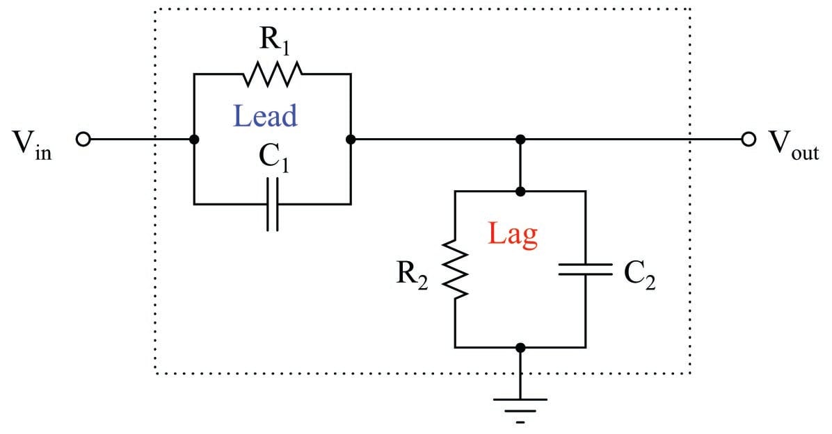
Each parallel RC subcircuit represents a time constant (\(\tau\)), one for lead and one for lag. The overall behavior of the network is determined by the relative magnitudes of these two time constants. Which ever time constant is larger, determines the overall characteristic of the network.
If the two time constant values are equal to each other (\(\tau_{lead} = \tau_{lag}\)), then the circuit performs no dynamic compensation at all, simply passing the input signal to the output with no change except for some attenuation:
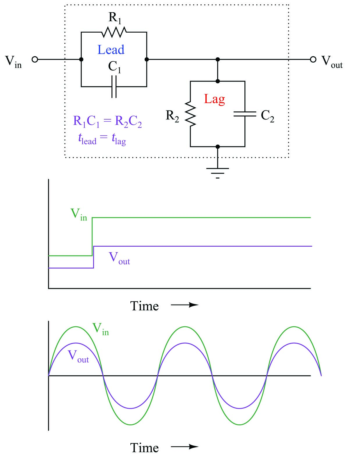
A square wave signal entering this network will exit the network as a square wave. If the input signal is sinusoidal, the output will also be sinusoidal and in-phase with the input.
If the lag time constant exceeds the lead time constant (\(\tau_{lag} > \tau_{lead}\)), then the overall behavior of the circuit will be to introduce a first-order lag to the voltage signal:
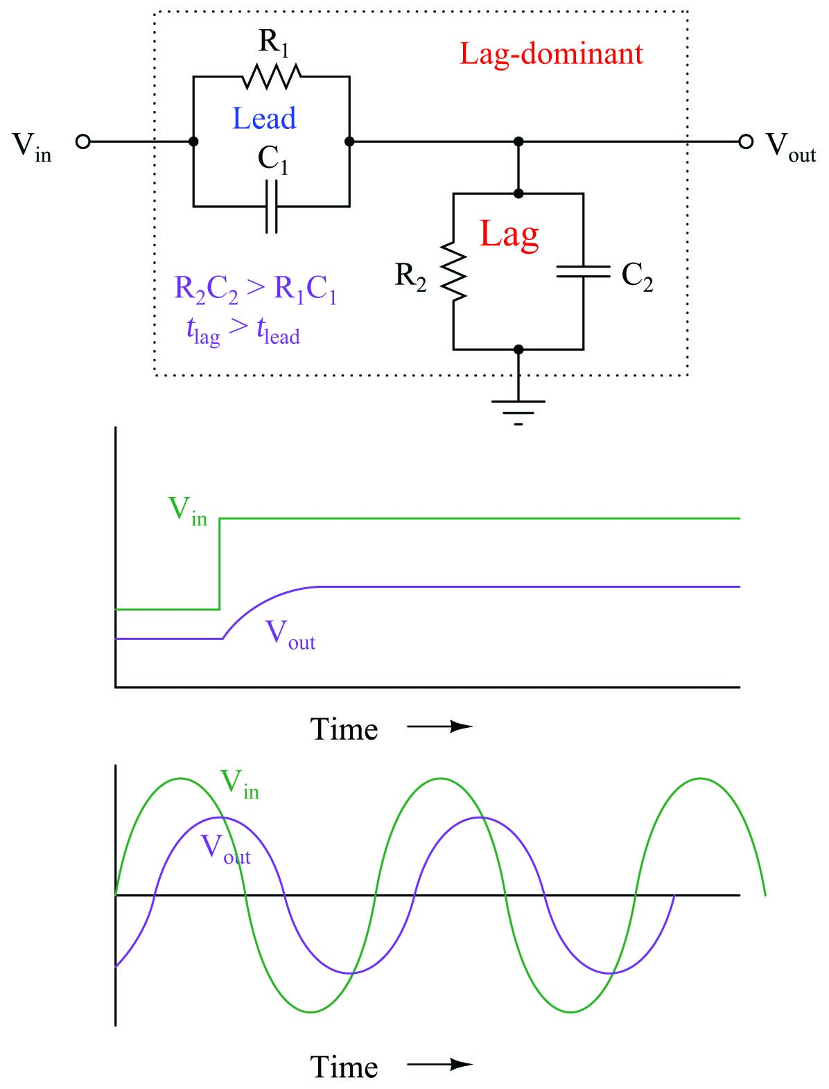
A square wave signal entering the network will exit the network as a sawtooth-shaped wave. A sinusoidal input will emerge sinusoidal, but with a lagging phase shift. This, in fact, is where the lag function gets its name: from the negative (“lagging”) phase shift it imparts to a sinusoidal input.
Conversely, if the lead time constant exceeds the lag time constant (\(\tau_{lead} > \tau_{lag}\)), then the overall behavior of the circuit will be to introduce a first-order lead to the voltage signal (a step-change voltage input will cause the output to “spike” and then settle to a steady-state value):
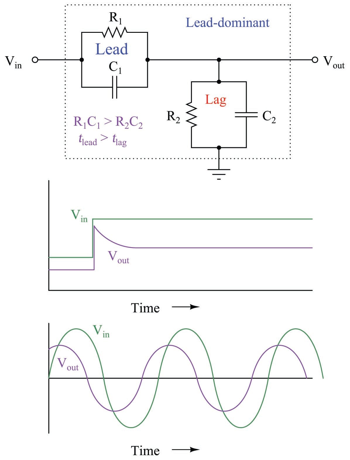
A square wave signal entering the network will exit the network with sharp transients on each leading edge. A sinusoidal input will emerge sinusoidal, but with a leading phase shift. Not surprisingly, this is where the lead function gets its name: from the positive (“leading”) phase shift it imparts to a sinusoidal input.
This exact form of lead/lag circuit finds application in a context far removed from process control: compensation for coaxial cable capacitance in a \(\times\)10 oscilloscope probe. Such probes are used to extend the voltage measurement range of standard oscilloscopes, and/or to increase the impedance of the instrument for minimal loading effect on sensitive electronic circuits. Using a \(\times\)10 probe, an oscilloscope will display a waveform that is \(1 \over 10\) the amplitude of the actual signal, and present ten times the normal impedance to the circuit under test.
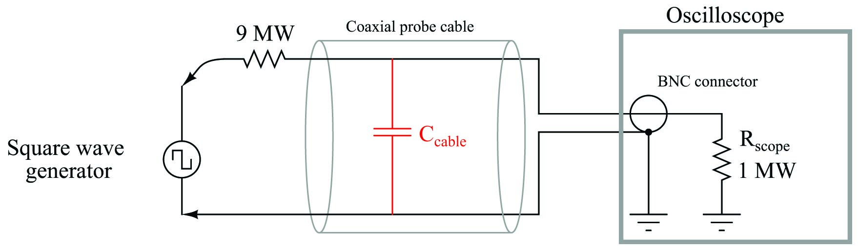
If a 9 M\(\Omega\) resistor is connected in series with a standard oscilloscope input (having an input impedance of 1 M\(\Omega\)) to create a 10:1 voltage division ratio, problems will result from the cable capacitance connecting the probe to the oscilloscope input. What should display as a square-wave input instead looks “rounded” by the effect of capacitance in the coaxial cable and at the oscilloscope input:
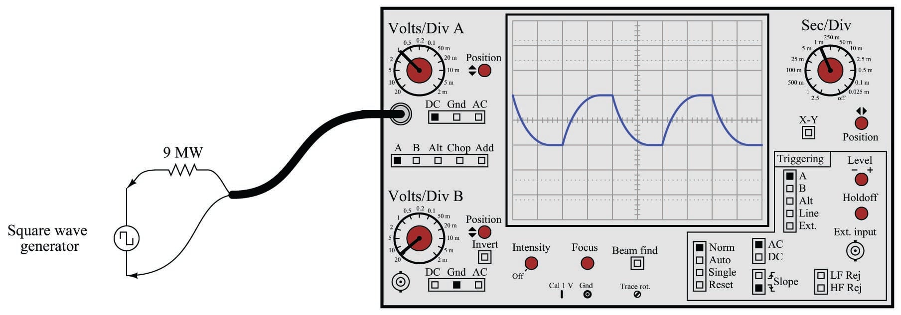
The reason for this is signal distortion the combined effect of the 9 M\(\Omega\) resistor and the cable’s natural capacitance forming an RC network:
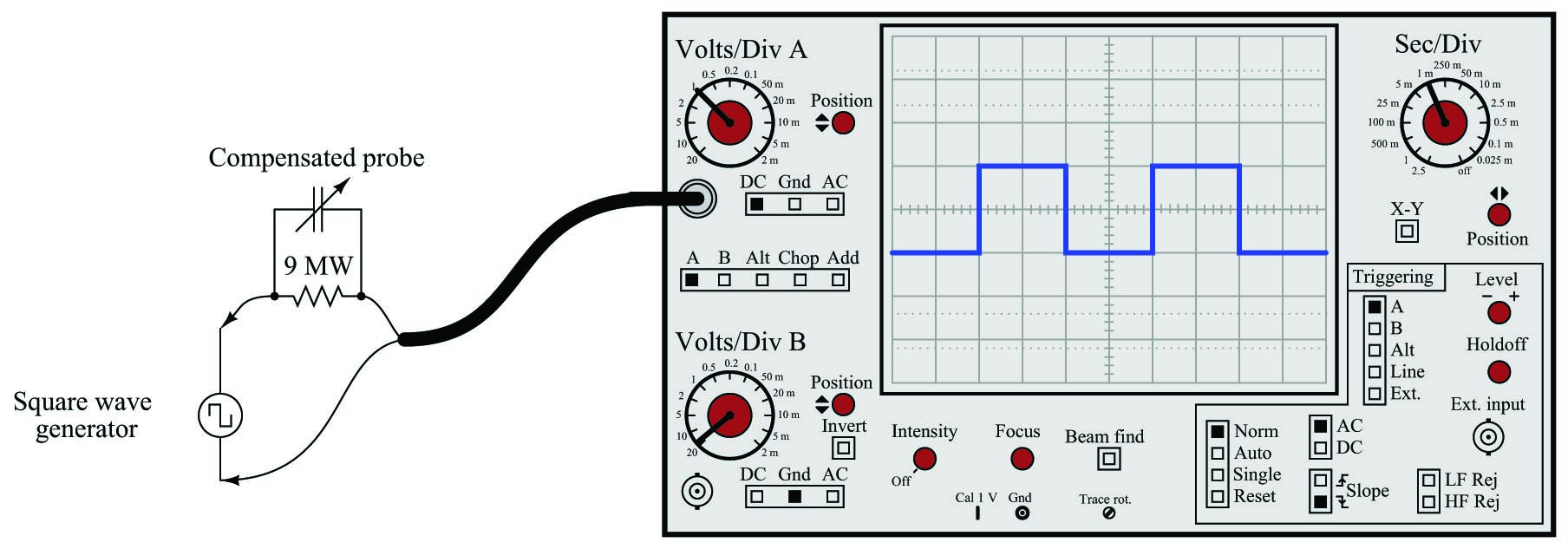
A simple solution to this problem is to build the 10:1 probe with a variable capacitor connected in parallel across the 9 M\(\Omega\) resistor. The combination of the 9 M\(\Omega\) resistor and this capacitor creates a lead network to cancel out the effects of the lag caused by the cable capacitance and 1 M\(\Omega\) oscilloscope impedance in parallel. When the capacitor is properly adjusted, the oscilloscope will accurately show the shape of any waveform at the probe tip, including square waves:
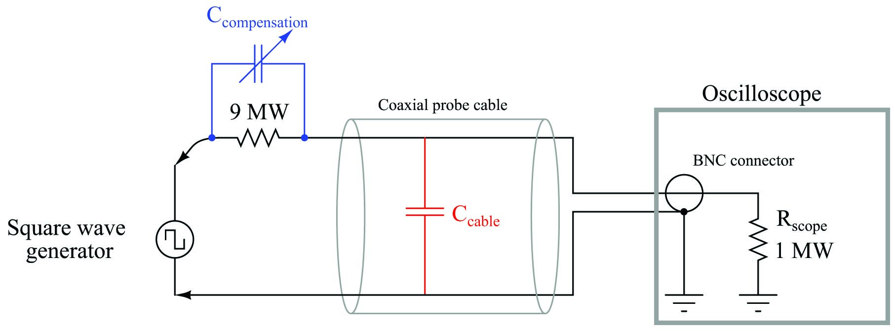
If we re-draw this compensated probe circuit to show the resistor pair and the capacitor pair both working as 10:1 voltage dividers, it becomes clearer to see how the two divider circuits work in parallel with each other to provide the same 10:1 division ratio only if the component ratios are properly proportioned:
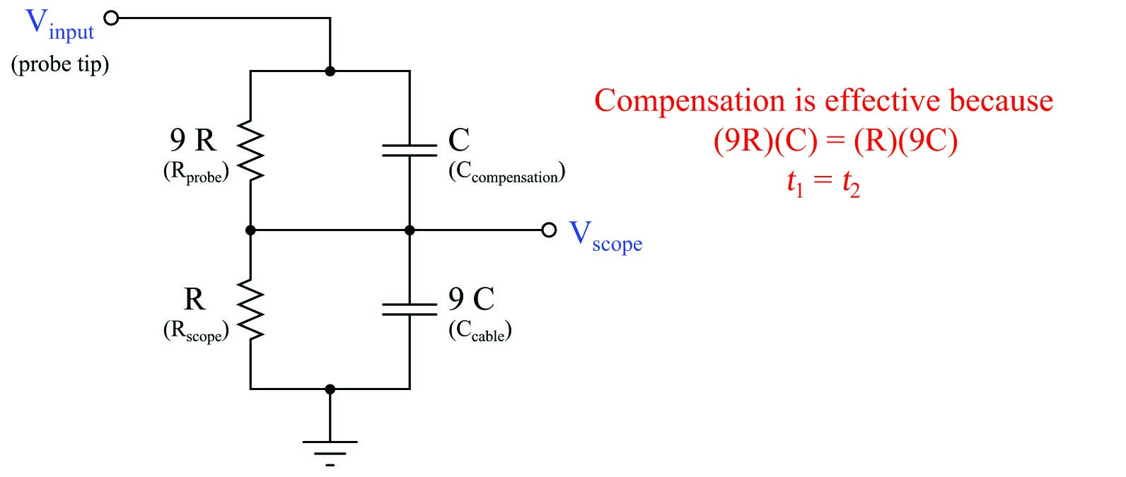
The series resistor pair forms an obvious 10:1 division ratio, with the smaller of the two resistors being in parallel with the oscilloscope input. The upper resistor, being 9 times larger in resistance value, drops 90% of the voltage applied to the probe tip. The series capacitor pair forms a less obvious 10:1 division ratio, with the cable capacitance being the larger of the two. Recall that the reactance of a capacitor to an AC voltage signal is inversely related to capacitance: a larger capacitor will have fewer ohms of reactance for any given frequency according to the formula \(X_C = { 1 \over {2 \pi f C}}\). Thus, the capacitive voltage divider network has the same 10:1 division ratio as the resistive voltage divider network, even though the capacitance ratios may look “backward” at first glance.
If the compensation capacitor is adjusted to an excessive value, the probe will overcompensate for lag (too much lead), resulting in a “spiked” waveform on the oscilloscope display with a perfect square-wave input:
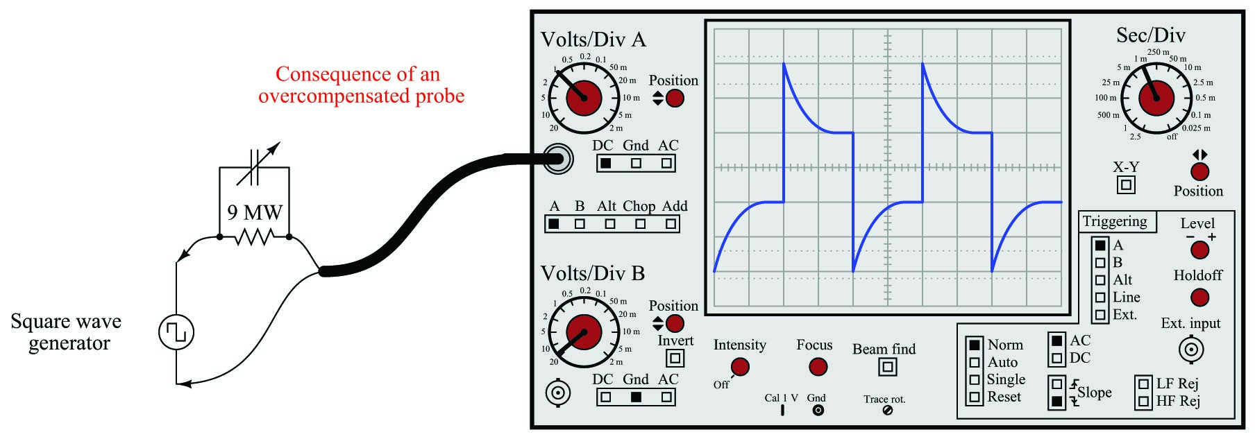
With the probe’s compensating capacitor exhibiting an excessive amount of capacitance, the capacitive voltage divider network has a voltage division ratio less than 10:1. This is why the waveform “spikes” on the leading edges: the capacitive divider dominates the network’s response in the short term, producing a voltage pulse at the oscilloscope input greater than it should be (divided by some ratio less than 10). Soon after the leading edge of the square wave passes, the capacitors’ effects will wane, leaving the resistors to establish the voltage division ratio on their own. Since the two resistors have the proper 10:1 ratio, this causes the oscilloscope’s signal to “settle” to its proper value over time. Thus, the waveform “spikes” too far at each leading edge and then decays to its proper amplitude over time.
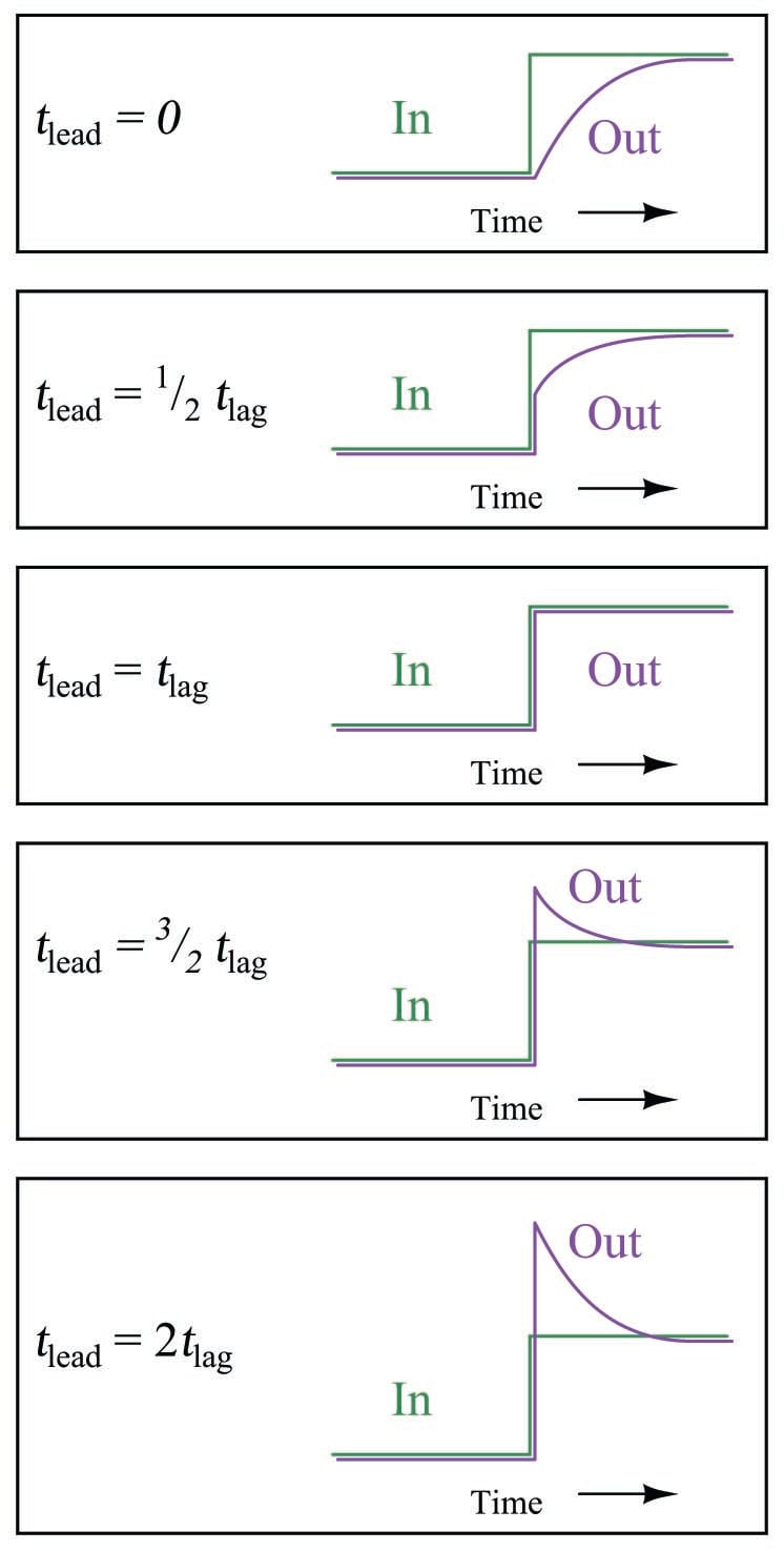
While undesirable in the context of oscilloscope probes, this is precisely the effect we desire in a process control lead function. The purpose of a lead/lag function is to provide a signal gain that begins at some initial value, then “settles” at another value over time. This way, sudden changes in the feedforward signal will either be amplified or attenuated for a short duration to compensate for lags in other parts of the control system, while the steady-state gain of the feedforward loop remains at some other value necessary for long-term stability. For a lag function, the initial gain is less than the final gain; for a lead function, the initial gain exceeds the final gain. If the lead and lag time constants are set equal to each other, the initial and final gains will likewise be equal, with the function exhibiting a constant gain at all times.
Although lead-lag functions for process control systems may be constructed from analog electronic components, modern systems implement the function arithmetically using digital microprocessors. A typical time-domain equation describing a digital lead/lag function block’s output response (\(y\)) to an input step-change from zero (0) to magnitude \(x\) over time (\(t\)) is as follows:
\[y = x \left(1 + {{{\tau_{lead} - \tau_{lag}} \over \tau_{lag} \> e^{t \over \tau_{lag} }}} \right)\]
As you can see, if the two time constants are set equal to each other (\(\tau_{lead} = \tau_{lag}\)), the second term inside the parentheses will have a value of zero at all times, reducing the equation to \(y = x\). If the lead time constant exceeds the lag time constant (\(\tau_{lead} > \tau_{lag}\)), then the fraction will begin with a positive value and decay to zero over time, giving us the “spike” response we expect from a lead function. Conversely, if the lag time constant exceeds the lead (\(\tau_{lag} > \tau_{lead}\)), the fraction will begin with a negative value at time = 0 (the beginning of the step-change) and decay to zero over time, giving us the “sawtooth” response we expect from a lag function.
It should also be evident from an examination of this equation that the “decay” time of the lead/lag function is set by the lag time constant (\(\tau_{lag}\)). Even if we just need the function to produce a “lead” response, we must still properly set \(\tau_{lag}\) in order for the lead response to decay at the correct rate for our control system. The intensity of the lead function (i.e. how far it “spikes” when presented with a step-change in input signal) varies with the ratio \(\tau_{lead} \over \tau_{lag}\), but the duration of the “settling” following that step-change is entirely set by \(\tau_{lag}\).
To summarize the behavior of a lead/lag function:
- If \(\tau_{lead} = \tau_{lag}\), the lead/lag function will simply pass the input signal through to the output (no lead or lag action at all)
- If \(\tau_{lead} = 0\), the lead/lag function will provide a pure lag response with a final gain of unity and a time constant of \(\tau_{lag}\)
- If \(\tau_{lead} = 2 (\tau_{lag})\), the lead/lag function will provide a lead response with an initial gain of 2, a final gain of unity, and a time constant of \(\tau_{lag}\)