 Facebook
 Google
 GitHub
 Linkedin
Limit, Selector, and Override Controls
Another category of control strategies involves the use of signal relays or function blocks with the ability to switch between different signal values, or re-direct signals to new pathways. Such functions are useful when we need a control system to choose between multiple signals of differing value in order to make the best control decisions.
The “building blocks” of such control strategies are special relays (or function blocks in a digital control system) shown here:

High-select functions output whichever input signal has the greatest value. Low-select functions do just the opposite: output whichever input signal has the least value. “Greater-than” and “Less than” symbols mark these two selector functions, respectively, and each type may be equipped to receive more than two input signals.
Sometimes you will see these relays represented in P&IDs simply by an inequality sign in the middle of the large bubble, rather than off to the side in a square. You should bear in mind that the location of the input lines has no relationship at all to the direction of the inequality symbol – e.g., it is not as though a high-select relay looks for the input on the left side to be greater than the input on the right. Note the examples shown below, complete with sample signal values:

High-limit and low-limit functions are similar to high- and low-select functions, but they only receive one input each, and the limit value is a parameter programmed into the function rather than received from another source. The purpose of these functions is to place a set limit on how high or how low a signal value is allowed to go before being passed on to another portion of the control system. If the signal value lies within the limit imposed by the function, the input signal value is simply passed on to the output with no modification.
Like the select functions, limit functions may appear in diagrams with nothing more than the limit symbol inside the bubble, rather than being drawn in a box off to the side:

Rate limit functions place a maximum rate-of-change limit on the input signal, such that the output signal will follow the input signal precisely until and unless the input signal’s rate-of-change over time (\(dx \over dt\)) exceeds the pre-configured limit value. In that case, the relay still produces a ramping output value, but the rate of that ramp remains fixed at the limit \(dx \over dt\) value no matter how fast the input keeps changing. After the output value “catches up” with the input value, the function once again will output a value precisely matching the input unless the input begins to rise or fall at too fast a rate again.
Limit controls
A common application for select and limit functions is in cascade control strategies, where the output of one controller becomes the setpoint for another. It is entirely possible for the primary (master) controller to call for a setpoint that is unreasonable or unsafe for the secondary (slave) to attain. If this possibility exists, it is wise to place a limit function between the two controllers to limit the cascaded setpoint signal.
In the following example, a cascade control system regulates the temperature of molten metal in a furnace, the output of the master (metal temperature) controller becoming the setpoint of the slave (air temperature) controller. A high limit function limits the maximum value this cascaded setpoint can attain, thereby protecting the refractory brick of the furnace from being exposed to excessive air temperatures:

It should be noted that although the different functions are drawn as separate bubbles in the P&ID, it is possible for multiple functions to exist within one physical control device. In this example, it is possible to find a controller able to perform the functions of both PID control blocks (master and slave) and the high limit function as well. It is also possible to use a distributed technology such as FOUNDATION Fieldbus to place all control functions inside field instruments, so only three field instruments exist in the loop: the air temperature transmitter, the metal temperature transmitter, and the control valve (with a Fieldbus positioner).
This same control strategy could have been implemented using a low select function block rather than a high limit:

Here, the low-select function selects whichever signal value is lesser: the setpoint value sent by the master temperature controller, or the maximum air temperature limit value sent by the hand indicating controller (HIC – sometimes referred to as a manual loading station).
An advantage of this latter approach over the former might be ease of limit value changes. With a pre-configured limit value residing in a high-limit function, it might be that only qualified maintenance people have access to changing that value. If the decision of the operations department is to have the air temperature limit value easily adjusted by anyone, the latter control strategy’s use of a manual loading station would be better suited1017.
Another detail to note in this system is the possibility of integral windup in the master controller in the event that the high setpoint limit takes effect. Once the high-limit (or low-select) function secures the slave controller’s remote setpoint at a fixed value, the master controller’s output is no longer controlling anything: it has become decoupled from the process. If, when in this state of affairs, the metal temperature is still below setpoint, the master controller’s integral action will “wind up” the output value over time with absolutely no effect, since the slave controller is no longer following its output signal. If and when the metal temperature reaches setpoint, the master controller’s output will likely be saturated at 100% due to the time it spent winding up. This will cause the metal temperature to overshoot setpoint, as a positive error will be required for the master controller’s integral action to wind back down from saturation.
[override_windup]
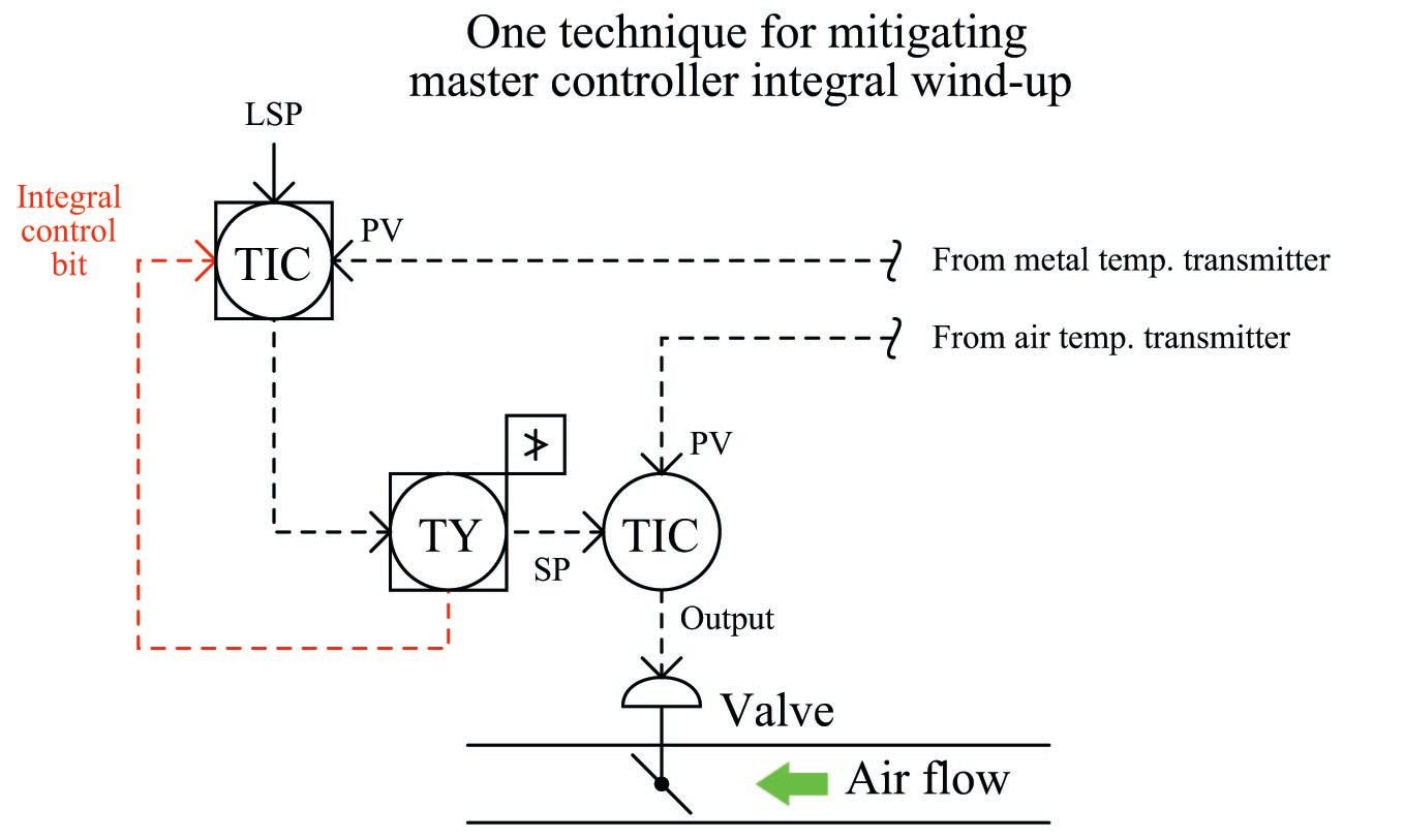
A relatively easy solution to this problem is to configure the master controller to stop integral action when the high limit relay engages. This is easiest to do if the master PID and high limit functions both reside in the same physical controller. Many digital limit function blocks generate a bit representing the state of that block (whether it is passing the input signal to the output or limiting the signal at the pre-configured value), and some PID function blocks have a boolean input used to disable integral action. If this is the case with the function blocks comprising the high-limit control strategy, it may be implemented like this:
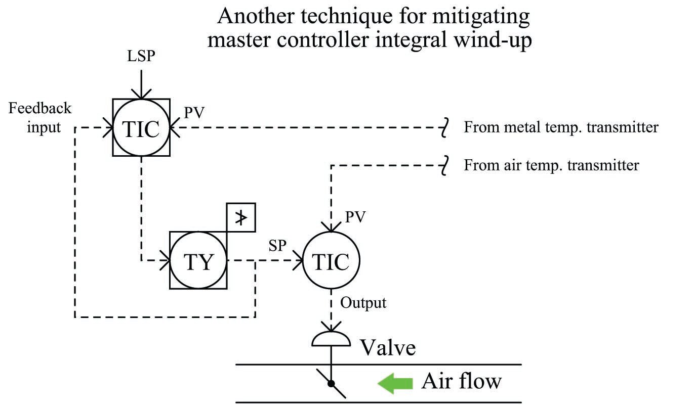
Another method used to prevent integral windup is to make use of the feedback input available on some PID function blocks. This is an input used to calculate the integral term of the PID equation. In the days of pneumatic PID controllers, this option used to be called external reset. Normally connected to the output of the PID block, if connected to the output of the high-limit function it will let the controller know whether or not any attempt to wind up the output is having an effect. If the output has been de-selected by the high-limit block, integral windup will cease:
Limit control strategies implemented in FOUNDATION Fieldbus instruments use the same principle, except that the concept of a “feedback” signal sending information backwards up the function block chain is an aggressively-applied design philosophy throughout the FOUNDATION Fieldbus standard. Nearly every function block in the Fieldbus suite provides a “back calculation” output, and nearly every function block accepts a “back calculation” input from a downstream block. The “Control Selector” (CS) function block specified in the FOUNDATION Fieldbus standard provides the limiting function we need between the master and slave controllers. The BKCAL_OUT signal of this selector block connects to the master controller’s BKCAL_IN input, making the master controller aware of its selection status. If ever the Control Selector function block de-selects the master controller’s output, the controller will immediately know to halt integral action:

This same “back calculation” philosophy – whereby the PID algorithm is aware of how another function is limiting or over-riding its output – is also found in some programmable logic controller (PLC) programming conventions. The Allen-Bradley Logix5000 series of PLCs, for example, provides a tieback variable to force the PID function’s output to track the overriding function. When the “tieback” variable is properly used, it allows the PID function to bumplessly transition from the “in-control” state to the “overridden” state.
Selector controls
In the broadest sense, a “selector” control strategy is where one signal is selected from multiple signals in a system to perform a measurement control function. In the context of this book and this chapter, I will use the term “selector” to reference automatic selection among multiple measurement or setpoint signals. Selection between multiple controller output signals will be explored in the next subsection, under the term “override” control.
Perhaps one of the simplest examples of a selector control strategy is where we must select a process variable signal from multiple transmitters. For example, consider this chemical reactor, where the control system must throttle the flow of coolant to keep the hottest measured temperature at setpoint, since the reaction happens to be exothermic (heat-releasing)1018:

The high-select relay (TY-24) sends only the highest temperature signal from the three transmitters to the controller. The other two temperature transmitter signals are simply ignored.
Another use of selector relays (or function blocks) is for the determination of a median process measurement. This sort of strategy is often used on triple-redundant measurement systems, where three transmitters are installed to measure the exact same process variable, providing a valid measurement even in the event of transmitter failure.
The median select function may be implemented one of two ways using high- and low-select function blocks:

The left-hand selector strategy selects the highest value from each pair of signals (A and B, B and C, A and C), then selects the lowest value of those three primary selections. The right-hand strategy is exactly opposite – first selecting the lowest value from each input pair, then selecting the highest of those values – but it still accomplishes the same function. Either strategy outputs the middle value of the three input signals1019.
Although either of these methods of obtaining a median measurement requires four signal selector functions, it is quite common to find function blocks available in control systems ready to perform the median select function all in a single block. The median-select function is so common to redundant sensor control systems that many control system manufacturers provide it as a standard function unto itself:

This is certainly true in the FOUNDATION Fieldbus standard, where two standardized function blocks are capable of this function, the CS (Control Selector) and the ISEL (Input Selector) blocks:

Of these two Fieldbus function blocks, the latter (ISEL) is expressly designed for selecting transmitter signals, whereas the former (CS) is best suited for selecting controller outputs with its “back calculation” facilities designed to modify the response of all de-selected controllers. Using the terminology of this book section, the ISEL function block is best suited for selector strategies, while the CS function block is ideal for limit and override strategies (discussed in the next section).
If receiving three “good” inputs, the ISEL function block will output the middle (median) value of the three. If one of the inputs carries a “bad” status1020, the ISEL block outputs the averaged value of the remaining two (good) inputs. Note how this function block also possesses individual “disable” inputs, giving external boolean (on/off) signals the ability to disable any one of the transmitter inputs to this block. Thus, the ISEL function block may be configured to de-select a particular transmitter input based on some programmed condition other than internal diagnostics.
If receiving four “good” inputs, the ISEL function block normally outputs the average value of the two middle (median) signal values. If one of the four inputs becomes “bad” is disabled, the block behaves as a normal three-input median select.
A general design principle for redundant transmitters is that you never install exactly two transmitters to measure the same process variable. Instead, you should install three (minimum). The problem with having two transmitters is a lack of information for “voting” if the two transmitters happen to disagree. In a three-transmitter system, the function blocks may select the median signal value, or average the “best 2 out of 3.” If there are just two transmitters installed, and they do not substantially agree with one another, it is anyone’s guess which one should be trusted1021.
A classic example of selectors in industrial control systems is that of a cross-limited ratio control strategy for air/fuel mixture applications. Before we explore the use of selector functions in such a strategy, we will begin by analyzing a simplified version of that strategy, where we control air and fuel flows to a precise ratio with no selector action at all:

Here, the fuel flow controller receives its setpoint directly from the firing command signal, which may originate from a human operator’s manual control or from the output of a temperature controller regulating temperature of the combustion-heated process. The air flow controller receives its setpoint from the fuel flow transmitter, with the calibrations of the air and fuel flow transmitters being appropriate to establish the proper air:fuel flow ratio when the transmitters register equally. From the perspective of the air flow controller, fuel flow is the wild flow while air flow is the captive flow.
There is a problem with this control system that may not be evident upon first inspection: the air:fuel ratio will tend to vary as the firing command signal increases or decreases in value over time. This is true even if the controllers are well-tuned and the air:fuel ratio remains well-controlled under steady-state conditions. The reason for this is linked to the roles of “wild” and “captive” flows, fuel and air flow respectively. Since the air flow controller receives its setpoint from the fuel flow transmitter, changes in air flow will always lag behind changes in fuel flow.
This sort of problem can be difficult to understand because it involves changes in multiple variables over time. A useful problem-solving technique to apply here is a “thought experiment,” coupled with a time-based graph to display the results. Our thought experiment consists of imagining what would happen if the firing command signal were to suddenly jump in value, then sketching the results on a graph.
If the firing command signal suddenly increases, the fuel flow controller responds by opening up the fuel valve, which after a slight delay results in increased fuel flow to the burner. This increased fuel flow signal gets sent to the setpoint input of the air flow controller, which in turn opens up the air valve to increase air flow proportionately. If the firing command signal suddenly decreased, the same changes in flow would occur in reverse direction but in the same chronological sequence, since the fuel flow change still “leads” the subsequent air flow change:

Inevitable delays in controller response, valve response, and flow transmitter response conspire to upset the air:fuel ratio during the times immediately following a step-change in firing command signal. When the firing command steps up, the fuel flow increases before the air flow, resulting in a short time when the burner runs “rich” (too much fuel, not enough air). When the firing command steps down, the fuel flow decreases before the air flow, resulting in a short time when the burner runs “lean” (too much air, not enough fuel). The scenario problem is dangerous because it may result in an explosion if an accumulation of unburnt fuel collects in a pocket of the combustion chamber and then ignites. The second scenario is generally not a problem unless the flame burns so lean that it risks blowing out.
The solution to this vexing problem is to re-configure the control scheme so that the air flow controller “takes the lead” whenever the firing command signal rises, and that the fuel flow controller “takes the lead” whenever the firing command signal falls. This way, any upsets in air:fuel ratio resulting from changes in firing command will always err on the side of a lean burn rather than a rich burn.
We may implement precisely this strategy by adding some signal selector functions to our ratio control system. The ratio is now cross-limited, where both measured flow rates serve as limiting variables to each other to ensure the air:fuel ratio can never be too rich:

Now, the air flow controller receives its setpoint either directly from the firing command signal or from the fuel flow transmitter, whichever signal is greater in value. The fuel flow controller receives its setpoint either directly from the firing command signal or from the air flow transmitter, whichever signal is least in value. Thus, the air flow controller “takes the lead” and makes fuel flow the “captive” variable when the firing command signal rises. Conversely, the fuel flow controller “takes the lead” and makes air flow the “captive” variable when the firing command signal falls. Instead of having the roles of “wild” and “captive” flows permanently assigned, these roles switch depending on which way the firing command signal changes.
Examining the response of this cross-limited system to sudden changes in firing command signal, we see how the air flow controller takes the lead whenever the firing rate signal increases, and how the fuel flow controller takes the lead whenever the firing rate signal decreases:

In both transient scenarios, the mixture runs lean (safe) rather than rich (dangerous). Of course, care must be taken to ensure the firing rate signal never steps up or down so quickly that the flame runs lean enough to blow out (i.e. the mixture becomes much too lean during a transient “step-change” of the firing rate signal). If this is a problem, we may fix it by installing rate-limiting functions in the firing command signal path, so that the firing command signal can never rise or fall too rapidly.
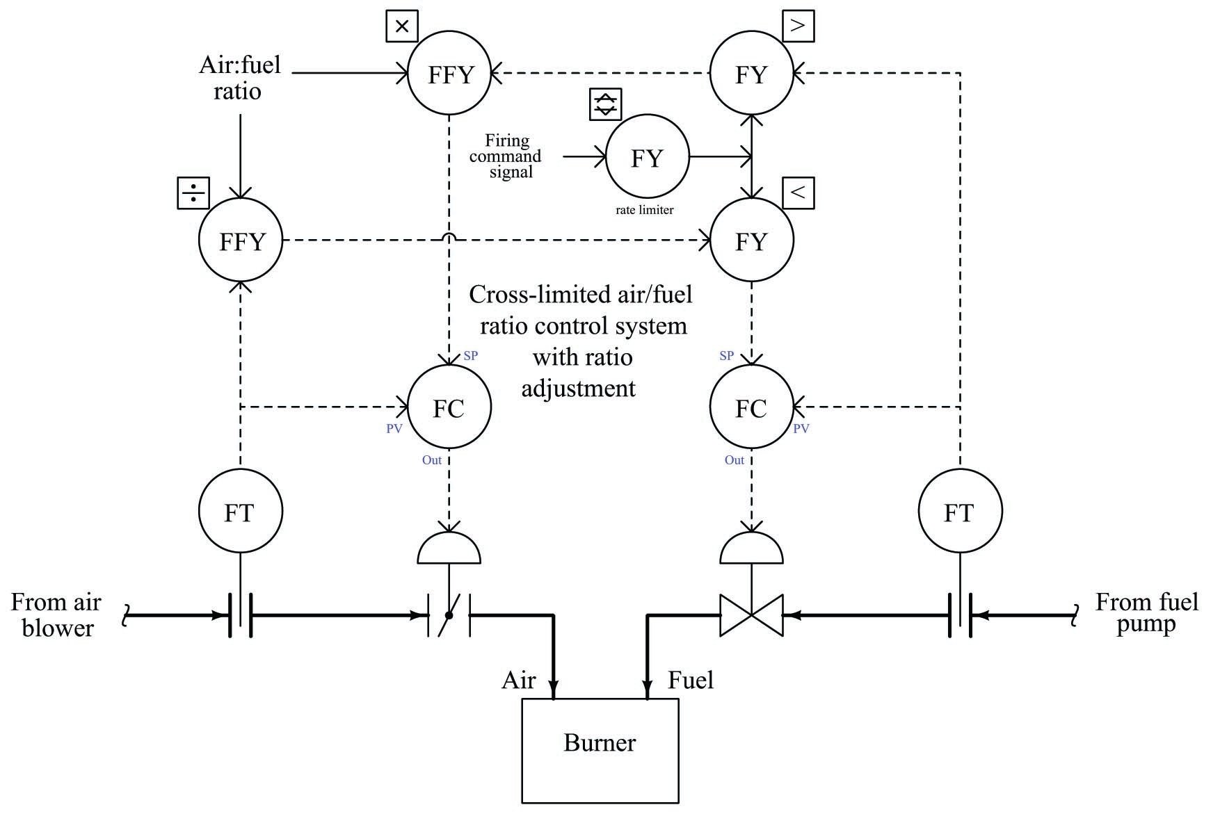
A realistic cross-limited ratio control system also incorporates a means to adjust the air:fuel ratio without having to re-range the air and/or fuel flow transmitters. Such ratio adjustment may be achieved by the insertion of a “multiplying” function between one of the selectors and a controller setpoint, plus a “dividing” function to return that scaled flow to a normalized value for cross-limiting.
The complete control strategy looks something like this, complete with cross-limiting of air and fuel flows, rate-limiting of the firing command signal, and adjustable air:fuel ratio:
Override controls
An “override” control strategy involves a selection between two or more controller output signals, where only one controller at a time gets the opportunity to exert control over a process. All other “de-selected” controllers are thus overridden by the selected controller.
The general concept of override control is easily understood by appeal to a human example. Cargo truck drivers must monitor and make control decisions on a wide number of variables, including diesel engine operating parameters and road rules. A truck driver needs to keep a close watch on the exhaust gas temperature of the truck engine: a leading indicator of impending engine damage (if exhaust temperature exceeds a pre-determined limit established by the engine manufacturer). The same truck driver must also drive as fast as the law will allow on any given road in order to minimize shipping time and thereby maximize the amount of cargo transported over long periods of time. These two goals may become mutually exclusive when hauling heavy cargo loads up steep inclines, such as when ascending a mountain pass. The goal of avoiding engine damage necessarily overrides the goal of maintaining legal road speed in such conditions.
Imagine a diesel truck driver maintaining the legal speed limit on a highway, occasionally glancing at the EGT (Exhaust Gas Temperature) indicator in the instrument panel. Under normal operating conditions, the EGT should be well below the danger threshold for the engine. However, after pulling a full load up a mountain pass and noticing the EGT approach the high operating limit, the truck driver makes the decision to regulate the engine’s power based on EGT rather than road speed. In other words, the legal speed limit is no longer the “setpoint” to control to, and EGT now is.
If we were to model the truck driver’s decision-making processes in industrial instrumentation terms, it would look something like this:

Which ever control decision calls for the least engine power output, “wins the vote” to control the engine’s power.
As is the case with limit and selector control strategies, a “select” function is used to choose one signal from multiple signals. The difference here is that the signals being selected are both controller outputs rather than transmitter (measurement) or setpoint signals. Both controllers are still active, but only one at a time will have any actual control over the process.
This model maps well to the truck driver analogy. Despite having “overridden” the goal of maintaining legal road speed in favor of maintaining a safe engine exhaust temperature, the driver is still thinking about road speed. In fact, if the driver happens to be behind schedule, you can be absolutely sure the goal of maintaining the highway speed limit has not been forgotten! In fact, the driver may become impatient as the long incline wears on, eager to make up lost time as soon as the opportunity allows. This is a potential problem for all override control systems: making sure the de-selected controller does not “wind up” (with integral action still active) while it has no control over the process.
An municipal example of override control is seen in this water pumping system, where a water pump is driven by a variable-speed1022 electric motor to draw water from a well and provide constant water pressure to a customer:
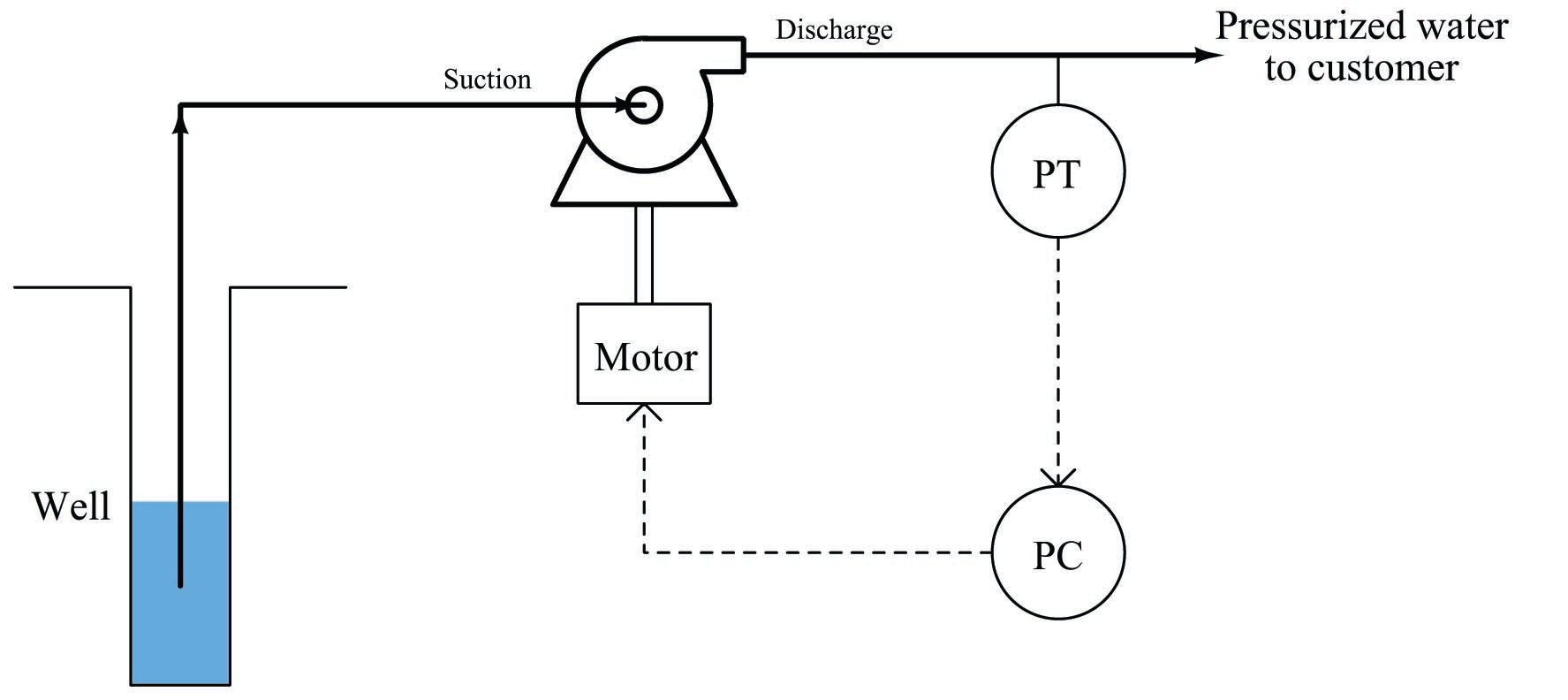
Incidentally, this is an excellent application for a variable-speed motor as the final control element rather than a control valve. Reducing pump speed in low-flow conditions will save a lot of energy over time compared to the energy that would be wasted by a constant-speed pump and control valve.
A potential problem with this system is the pump running “dry” if the water level in the well gets too low, as might happen during summer months when rainfall is low and customer demand is high. If the pump runs for too long with no water passing through it, the seals will become damaged. This will necessitate a complete shut-down and costly rebuild of the pump, right at the time customers need it the most.
One solution to this problem would be to install a level switch in the well, sensing water level and shutting off the electric motor driving the pump if the water level ever gets too low:

This may be considered a kind of “override” strategy, because the low-level switch over-rides the pressure controller’s command for the pump to turn. It is also a crude solution to the problem, for while it protects the pump from damage, it does so at the cost of completely shutting off water to customers. One way to describe this control strategy would be to call it a hard override system, suggesting the uncompromising action it will take to protect the pump.
A better solution to the dilemma would be to have the pump merely slow down as the well water level approaches a low-level condition. This way at least the pump could be kept running (and some amount of pressure maintained), decreasing demand on the well while maintaining curtailed service to customers and still protecting the pump from dry-running. This would be termed a soft override system.
We may create just such a control strategy by replacing the well water level switch with a level transmitter, connecting the level transmitter to a level controller, and using a low-select relay or function block to select the lowest-valued output between the pressure and level controllers. The level controller’s setpoint will be set at some low level above the acceptable limit for continuous pump operation:

If ever the well’s water level goes below this setpoint, the level controller will command the pump to slow down, even if the pressure controller is calling for a higher speed. The level controller will have overridden the pressure controller, prioritizing pump longevity over customer demand.
Bear in mind that the concept of a low-level switch completely shutting off the pump is not an entirely bad idea. In fact, it might be prudent to integrate such a “hard” shutdown control in the override control system, just in case something goes wrong with the level controller (e.g. an improperly adjusted setpoint or poor tuning) or the low-select function.
With two layers of safety control for the pump, this system provides both a “soft constraint” providing moderated action and a “hard constraint” providing aggressive action to protect the pump from dry operation:

In order that these two levels of pump protection work in the proper order, the level controller’s (LC) setpoint needs to be set to a higher value than the low level alarm’s (LAL) trip point.
A very important consideration for any override control strategy is how to manage integral windup. Any time a controller with any integral (reset) action at all is de-selected by the selector function, the integral term of the controller will have the tendency to wind up (or wind down) over time. With the output of that controller de-coupled from the final control element, it can have no effect on the process variable. Thus, integral control action – the purpose of which being to constantly drive the output signal in the direction necessary to achieve equality between process variable and setpoint – will work in vain to eliminate an error it cannot influence. If and when control is handed back to that controller, the integral action will have to spend time “winding” the other way to un-do what it did while it was de-selected.
Thus, override controls demand some form of integral windup limits that engage when a controller is de-selected. Methods of accomplishing this function are discussed in an earlier section on limit controls (section [override_windup] beginning on page ).
