 Facebook
 Google
 GitHub
 Linkedin
Non-contact Temperature Sensors
Virtually any mass above absolute zero temperature emits electromagnetic radiation (photons, or light) as a function of that temperature. This basic fact makes possible the measurement of temperature by analyzing the light emitted by an object. The Stefan-Boltzmann Law of radiated energy quantifies this fact, declaring that the rate of heat lost by radiant emission from a hot object is proportional to the fourth power of the absolute temperature:
\[{dQ \over dt} = e \sigma A T^4\]
Where,
\(dQ \over dt\) = Radiant heat loss rate (watts)
\(e\) = Emissivity factor (unitless)
\(\sigma\) = Stefan-Boltzmann constant (5.67 \(\times\) \(10^{-8}\) W / m\(^{2}\) \(\cdot\) K\(^{4}\))
\(A\) = Surface area (square meters)
\(T\) = Absolute temperature (Kelvin)
The primary advantage of non-contact thermometry (or pyrometry as high-temperature measurement is often referred) is rather obvious: with no need to place a sensor in direct contact with the process, a wide variety of temperature measurements may be made that are either impractical or impossible to make using any other technology.
A major disadvantage of non-contact thermometry is that it only reveals the surface temperature of an object. Sensing the thermal radiation emanated from a pipe, for instance, only tells you the surface temperature of that pipe and not the true temperature of the fluid within the pipe. Another example is when doctors use non-contact thermometry to assess irregularities in body temperature: what they detect is just skin temperature. While it may be true that “hot spots” beneath the surface of an object may be detectable this way, it is only because the surface temperature of that object differs as a consequence of the hot spot(s) beneath. If a hotter-than-normal region inside of an object fails to transfer enough thermal energy to the surface to manifest as a hotter surface temperature, that region will be invisible to non-contact thermometry.
It may surprise some readers to discover that non-contact pyrometry is nearly as old as thermocouple technology, the first non-contact pyrometer being constructed in 1892.
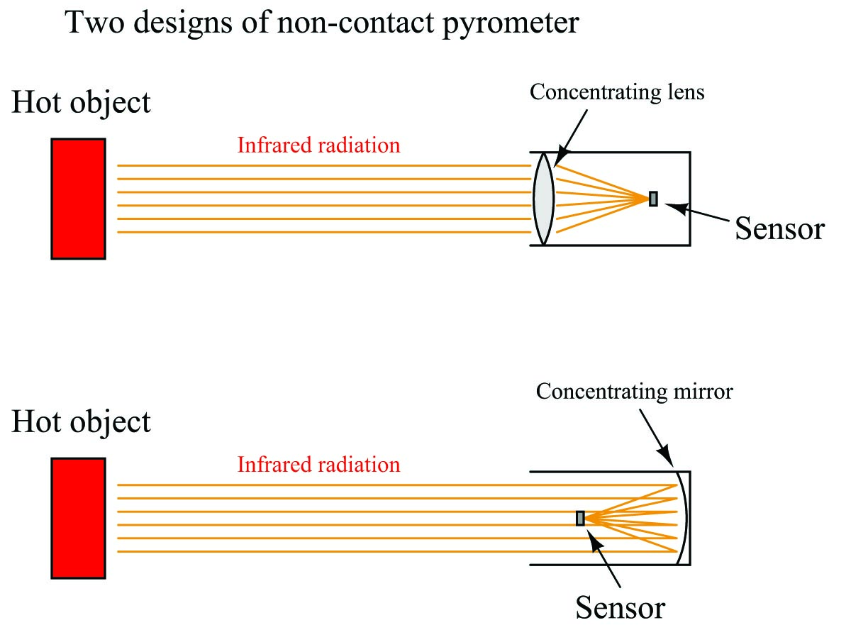
Concentrating pyrometers
A time-honored design for non-contact pyrometers is to concentrate incident light from the surface of a heated object onto a small temperature-sensing element. A rise in temperature at the sensor reveals the intensity of the infrared optical energy falling upon it, which as discussed previously is a function of the target object’s surface temperature (absolute temperature to the fourth power):
The fourth-power characteristic of Stefan-Boltzmann’s law means that a doubling of absolute temperature at the hot object results in sixteen times as much radiant energy falling on the sensor, and therefore a sixteen-fold increase in the sensor’s temperature rise over ambient. A tripling of target temperature (absolute) yields eighty one times as much radiant energy, and therefore an 81-fold increase in sensor temperature rise. This extreme nonlinearity limits the practical application of non-contact pyrometry to relatively narrow ranges of target temperature wherever good accuracy is required.
Thermocouples were the first type of sensor used in non-contact pyrometers, and they still find application in modern versions of the same technology. Since the sensor does not become nearly as hot as the target object, the output of any single thermocouple junction at the sensor area will be quite small. For this reason, instrument manufacturers often employ a series-connected array of thermocouples called a thermopile to generate a stronger electrical signal.
The basic concept of a thermopile is to connect multiple thermocouple junctions in series so their voltages will add:
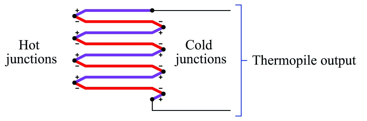
Examining the polarity marks of each junction (type E thermocouple wires are assumed in this example: chromel and constantan), we see that all the “hot” junctions’ voltages aid each other, as do all the “cold” junctions’ voltages. Like all thermocouple circuits, though, the each “cold” junction voltage opposes each the “hot” junction voltage. The example thermopile shown in this diagram, with four hot junctions and four cold junctions, will generate four times the potential difference that a single type E thermocouple hot/cold junction pair would generate, assuming all the hot junctions are at the same temperature and all the cold junctions are at the same temperature.
When used as the detector for a non-contact pyrometer, the thermopile is oriented so all the concentrated light falls on the hot junctions (the “focal point” where the light focuses to a small spot), while the cold junctions face away from the focal point to a region of ambient temperature. Thus, the thermopile acts like a multiplied thermocouple, generating more voltage than a single thermocouple junction could under the same temperature conditions.
A popular design of non-contact pyrometer manufactured for years by Honeywell was the Radiamatic, using ten thermocouple junction pairs arrayed in a circle. All the “hot” junctions were placed at the center of this circle where the focal point of the concentrated light fell, while all the “cold” junctions were situated around the circumference of the circle away from the heat of the focal point. A table of values showing the approximate relationship between target temperature and millivolt output for one model of Radiamatic sensing unit reveals the fourth-power function:
| Target temperature (K) | Millivolt output |
|---|---|
| 4144 K | 34.8 mV |
| 3866 K | 26.6 mV |
| 3589 K | 19.7 mV |
| 3311 K | 14.0 mV |
| 3033 K | 9.9 mV |
| 2755 K | 6.6 mV |
| 2478 K | 4.2 mV |
| 2200 K | 2.5 mV |
| 1922 K | 1.4 mV |
| 1644 K | 0.7 mV |
We may test the basic validity of the Stefan-Boltzmann law by finding the ratio of temperatures for any two temperature values in this table, raising that ratio to the fourth power, and seeing if the millivolt output signals for those same two temperatures match the new ratio. The operating theory here is that increases in target temperature will produce fourth-power increases in sensor temperature rise, since the sensor’s temperature rise should be a direct function of radiation power impinging on it.
For example, if we were to take 4144 K and 3033 K as our two test temperatures, we find that the ratio of these two temperature values is 1.3663. Raising this ratio to the fourth power gives us 3.485 for a predicted ratio of millivolt values. Multiplying the 3033 K millivoltage value of 9.9 mV by 3.485 gives us 34.5 mV, which is quite close to the value of 34.8 mV advertised by Honeywell:
\[{4144 \hbox{ K} \over 3033 \hbox{ K}} = 1.3663\]
\[\left({4144 \hbox{ K} \over 3033 \hbox{ K}}\right)^4 = 1.3663^4 = 3.485\]
\[(3.485)(9.9 \hbox{ mV}) \approx 34.8 \hbox{ mV}\]
If accuracy is not terribly important, and if the range of measured temperatures for the process is modest, we may take the millivoltage output of such a sensor and interpret it linearly. When used in this fashion, a non-contact pyrometer is often referred to as an infrared thermocouple, with the output voltage intended to connect directly to a thermocouple-input instrument such as an indicator, transmitter, recorder, or controller. An example of this usage is the OS-36 line of infrared thermocouples manufactured by Omega.
Infrared thermocouples are manufactured for a narrow range of temperature (most OS-36 models limited to a calibration span of 100 \(^{o}\)F or less), their thermopiles designed to produce millivolt signals corresponding to a standard thermocouple type (T, J, K, etc.) over that narrow range.
Distance considerations
An interesting and useful characteristic of non-contact pyrometers is that their calibration does not depend on the distance separating the sensor from the target object’s surface. This is counter-intuitive to anyone who has ever stood near an intense radiative heat source: standing in close proximity to a bonfire, for example, results in much hotter skin temperature than standing far away from it. Why wouldn’t a non-contact pyrometer register cooler target temperatures when it was far away, given the fact that infrared radiation from the object spreads out with increased separation distance? The fact that an infrared pyrometer does not suffer from this limitation is good for our purposes in measuring temperature, but it doesn’t seem to make sense at first.
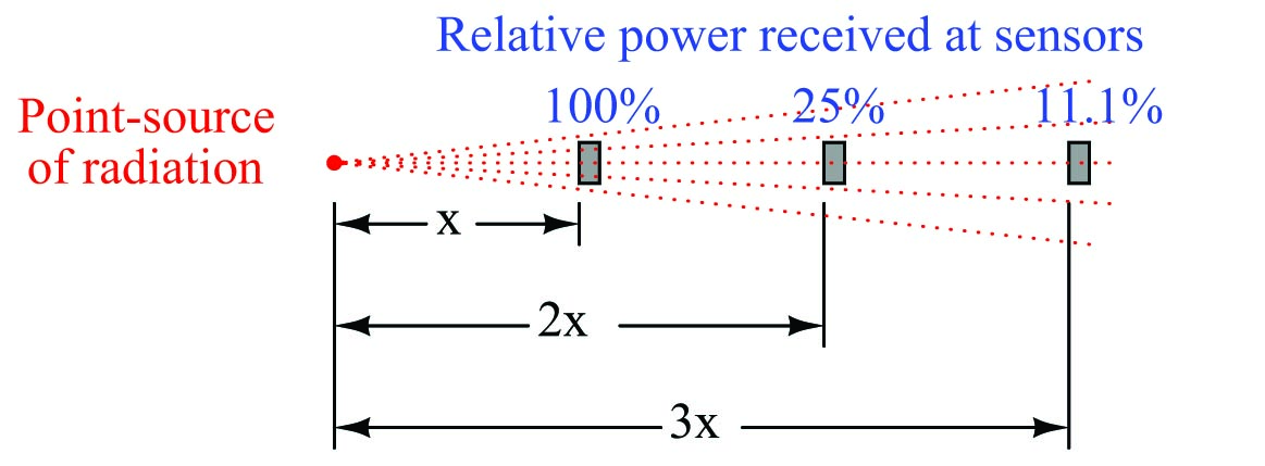
One key to understanding this paradox is to quantify the bonfire experience, where perceived temperature falls off with increased distance. In physics, this is known as the inverse square law: the intensity of radiation falling on an object from a point-source decreases with the square of the distance separating the radiation source from the object. Backing away to twice the distance from a bonfire results in a four-fold decrease in received infrared radiation; backing way to three times the distance results in a nine-fold decrease in received radiation.
Placing a sensor at three integer distances (\(x\), \(2x\), and \(3x\)) from a radiation point-source results in relative power levels of 100%, 25% (one-quarter), and 11.1% (one-ninth) falling upon the sensor at those locations, respectively:
This is a basic physical principle for all kinds of radiation, grounded in simple geometry. If we examine the radiation flux emanating from a point-source, we find that it must spread out as it travels in straight lines, and that the spreading-out happens at a rate defined by the square of the distance. An analogy for this phenomenon is to imagine a spherical latex balloon expanding as air is blown into it. The surface area of the balloon is proportional to the square of its radius. Likewise, the radiation flux emanating from a point-source spreads out in straight lines, in all directions, reaching a total area proportional to the square of the distance from the point (center). The total flux measured as a sphere will be the same no matter what the distance from the point-source, but the area it is divided over increases with the square of the distance, and so any object of fixed area backing away from a point-source of radiation encounters a smaller and smaller fraction of that flux.
If non-contact pyrometers really were “looking” at a point-source of infrared radiation, their signals would indeed decrease with distance. The saving grace here is that non-contact pyrometers are focused-optic devices, with a definite field of view, and that field of view should always be completely filled by the target object (assumed to be at a uniform temperature). As distance between the pyrometer and the target object changes, the cone-shaped field of view covers a surface area on that object proportional to the square of the distance Backing the pyrometer away to twice the distance increases the viewing area on the target object by a factor of four; backing away to three times the distance increases the viewing area nine times:
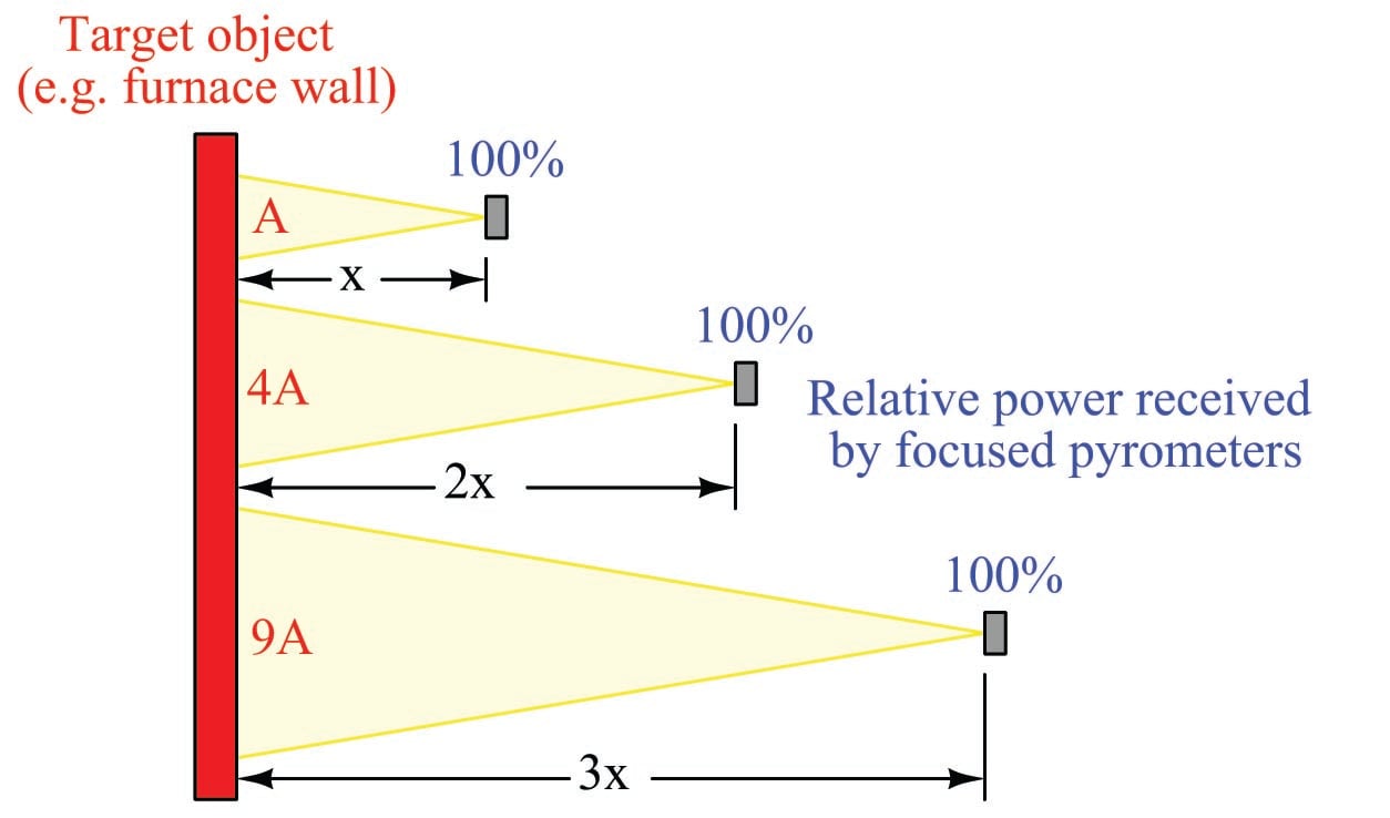
So, even though the inverse square law correctly declares that radiation emanating from the hot wall (which may be thought of as a collection of point-sources) decreases in intensity with the square of the distance, this attenuation is perfectly balanced by an increased viewing area of the pyrometer. Doubling the separation distance does result in the flux from any given point on the wall spreading out by a factor of four, but the pyrometer now sees four times as many similar points on the wall as it did previously. So long as all the points within the field of view are uniform in temperature, the result is a perfect cancellation with the pyrometer providing the exact same temperature measurement at any distance from the target.
If the sensor’s field of view expands far enough to capture objects other than the one whose temperature we intend to measure, measurement errors will result. The sensor will now yield a weighted average of all objects within its field of view, and so it is important to ensure that field is limited to cover just the object we intend to measure.
Non-contact sensor fields-of-view are typically specified either as an angle, as a distance ratio, or both. For example, the following illustration shows a non-contact temperature sensor with a 5:1 (approximately 11\(^{o}\)) field of view:
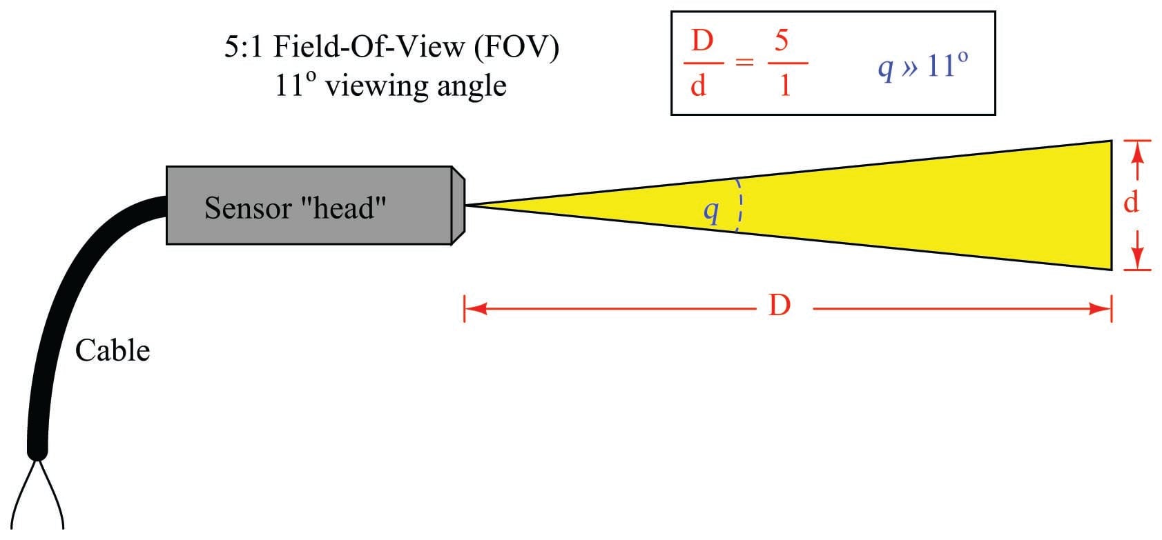
The mathematical relationship between viewing angle (\(\theta\)) and distance ratio (\(D/d\)) follows the tangent function:
\[{D \over d} = {1 \over {2 \tan \left({\theta \over 2}\right)}} \hskip 30pt \theta = 2 \tan^{-1} \left({d \over 2D}\right)\]
A sampling of common field-of-view distance ratios and approximate viewing angles appears in this table:
ratio & (approximate) \cr
| Distance | Angle | 1:1 | 53$^{o}$ |
|---|---|---|---|
| 2:1 | 30$^{o}$ | ||
| 3:1 | 19$^{o}$ | ||
| 5:1 | 11$^{o}$ | ||
| 7:1 | 8$^{o}$ | ||
| 10:1 | 6$^{o}$ |
A trigonometric explanation for these equations is shown in the following diagram, where the isosceles field-of-vision triangle is split into two “right” triangles, each one having an adjacent side length of \(D\) and an opposite side length of \(d/2\) for angle \(\theta/2\):
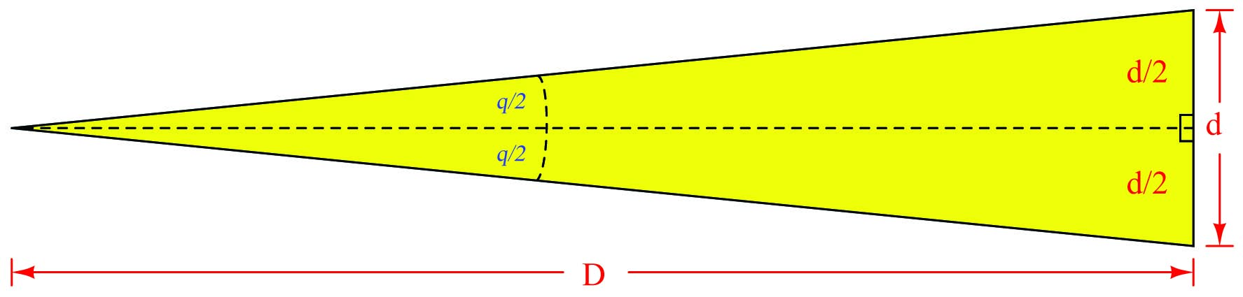
Since we know the tangent function is the ratio of opposite to adjacent side lengths for a right triangle, this means the tangent of the half-angle (\(\theta/2\)) will be equal to the ratio of the opposite side length (\(d/2\)) to the adjacent side length (\(D\)):
\[\tan \left( {\theta \over 2} \right) = {{d/2} \over D} = {d \over 2D}\]
Solving for the length ratio \(D/d\) is now just a matter of algebraically manipulating this equation:
\[\tan \left( {\theta \over 2} \right) = {d \over 2D}\]
\[{2D \over d} = {1 \over {\tan \left( {\theta \over 2} \right)}}\]
\[{D \over d} = {1 \over {2 \tan \left( {\theta \over 2} \right)}}\]
Solving for the viewing angle (\(\theta\)) requires another form of manipulation on the basic tangent equation, where we “un-do” the tangent function by using the inverse tangent (or “arctangent”) function:
\[\tan \left( {\theta \over 2} \right) = {d \over 2D}\]
\[\tan^{-1} \left[\tan \left( {\theta \over 2} \right) \right] = \tan^{-1} \left({d \over 2D}\right)\]
\[{\theta \over 2} = \tan^{-1} \left({d \over 2D}\right)\]
\[\theta = 2 \tan^{-1} \left({d \over 2D}\right)\]
Emissivity
Aside from their inherent nonlinearity, perhaps the main disadvantage of non-contact temperature sensors is their inaccuracy. The emissivity factor (\(e\)) in the Stefan-Boltzmann equation varies with the composition of a substance, but beyond that there are several other factors (surface finish, shape, etc.) that affect the amount of radiation a sensor will receive from an object. For this reason, emissivity is not a very practical way to gauge the effectiveness of a non-contact pyrometer. Instead, a more comprehensive measure of an object’s “thermal-optical measureability” is emittance.
A perfect emitter of thermal radiation is known as a blackbody. Emittance for a blackbody is unity (1), while emittance figures for any real object is a value between 1 and 0. The only certain way to know the emittance of an object is to test that object’s thermal radiation at a known temperature. This assumes we have the ability to measure that object’s temperature by direct contact, which of course renders void one of the major purposes of non-contact thermometry: to be able to measure an object’s temperature without having to touch it. Not all hope is lost, though: all we have to do is obtain an emittance value for that object one time, and then we may calibrate any non-contact pyrometer for that object’s particular emittance so as to measure its temperature in the future without contact.
Beyond the issue of emittance, other idiosyncrasies plague non-contact pyrometers. Objects also have the ability to reflect and transmit radiation from other bodies, which taints the accuracy of any non-contact device sensing the radiation from that body. An example of the former is trying to measure the temperature of a silver mirror using an optical pyrometer: the radiation received by the pyrometer is mostly from other objects, merely reflected by the mirror. An example of the latter is trying to measure the temperature of a gas or a clear liquid, and instead primarily measuring the temperature of a solid object in the background (through the gas or liquid).
Nevertheless, non-contact pyrometers have been and will continue to be useful in specific applications where other, contact-based temperature measurement techniques are impractical.
Thermal imaging
A very useful application of non-contact sensor technology is thermal imaging, where a dense array of infrared radiation sensors provides a graphic display of objects in its view according to their temperatures. Each object shown on the digital display of a thermal imager is artificially colored in the display on a chromatic scale that varies with temperature, hot objects typically registering as red tones and cold objects typically registering as blue tones. Thermal imaging is very useful in the electric power distribution industry, where technicians may inspect power line insulators and other objects at elevated potential for “hot spots” without having to make physical contact with those objects. Thermal imaging is also useful in performing “energy audits” of buildings and other heated structures, providing a means of revealing points of heat escape through walls, windows, and roofs. In such applications, relative differences in temperature are often more important to detect than specific temperature values. “Hot spots” readily appear on a thermal imager display, and may give useful data on the test subject even in the absence of accurate temperature measurement at any one spot.
Again, it is important to stress that thermal imaging only provides an assessment of the object’s surface temperature, and not the temperature within that object. Variations in surface temperature detectable by thermal imaging are a secondary effect of temperature variations within the object, and as such may not accurately depict the true thermal gradient(s) within the object.
A digital image taken with a thermal imaging instrument by maintenance personnel at a municipal water treatment facility shows “hot spots” on an electric motor. A color scale on the right-hand side of the image serves as a “legend” for interpreting color as temperature. In this particular shot, dark blue is 68.1 \(^{o}\)F and white is 152 \(^{o}\)F:
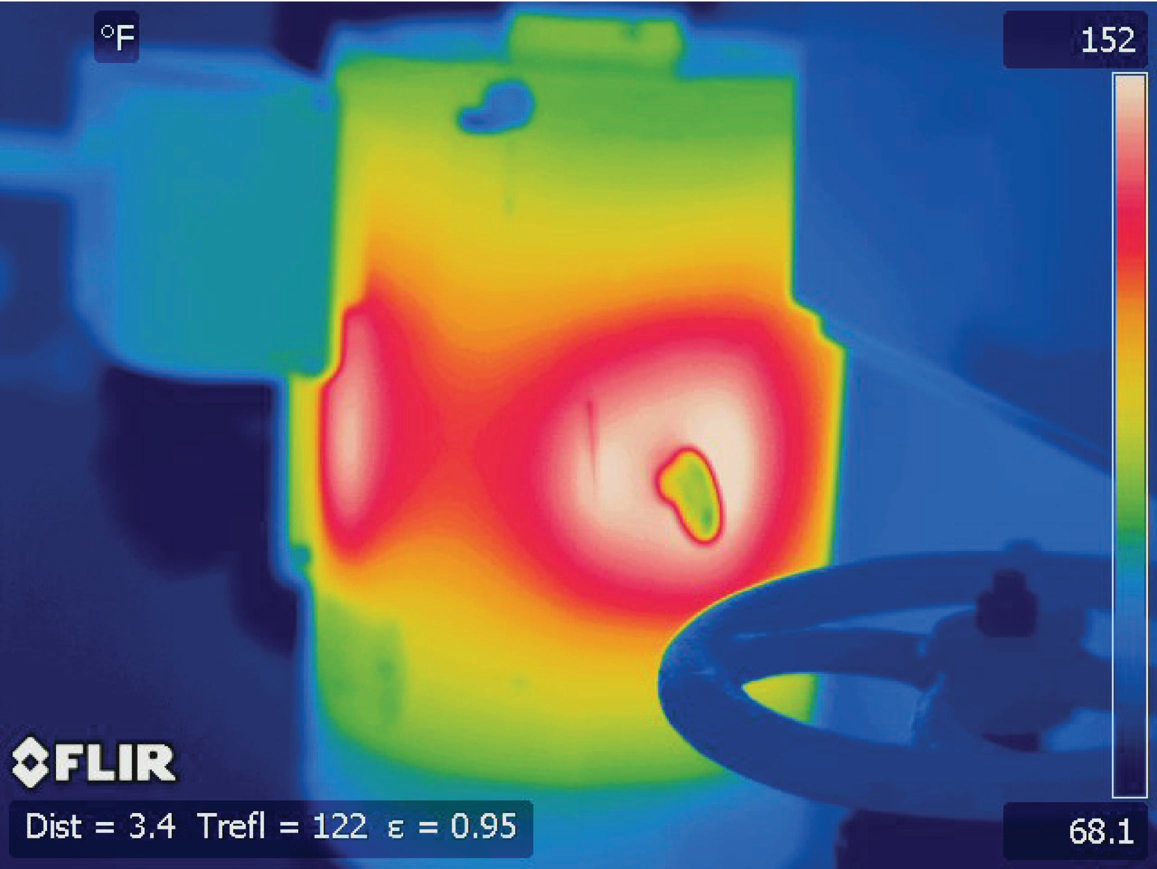
This particular electric motor is in a vertical orientation, with the electrical connection box in the upper-left corner and two prominent hot spots on both the near and the left-facing sides of the case. A manual valve handle appears in the foreground, silhouetted in dark blue against a lighter blue (warmer) background. A lifting “eye” on the motor case appears as a green (cooler) shape in the middle of a white (warmer) area. The two “hot spots” correspond directly to stator windings and magnetic pole faces inside the motor, which are close enough to the motor’s casing to cause variations in surface temperature.
Thermal imaging is particularly useful for detecting hot spots on equipment unsafe to directly touch, as is the case with many “live” electrical components. This next thermal image shows an operating three-phase motor starter (contactor and overload block):
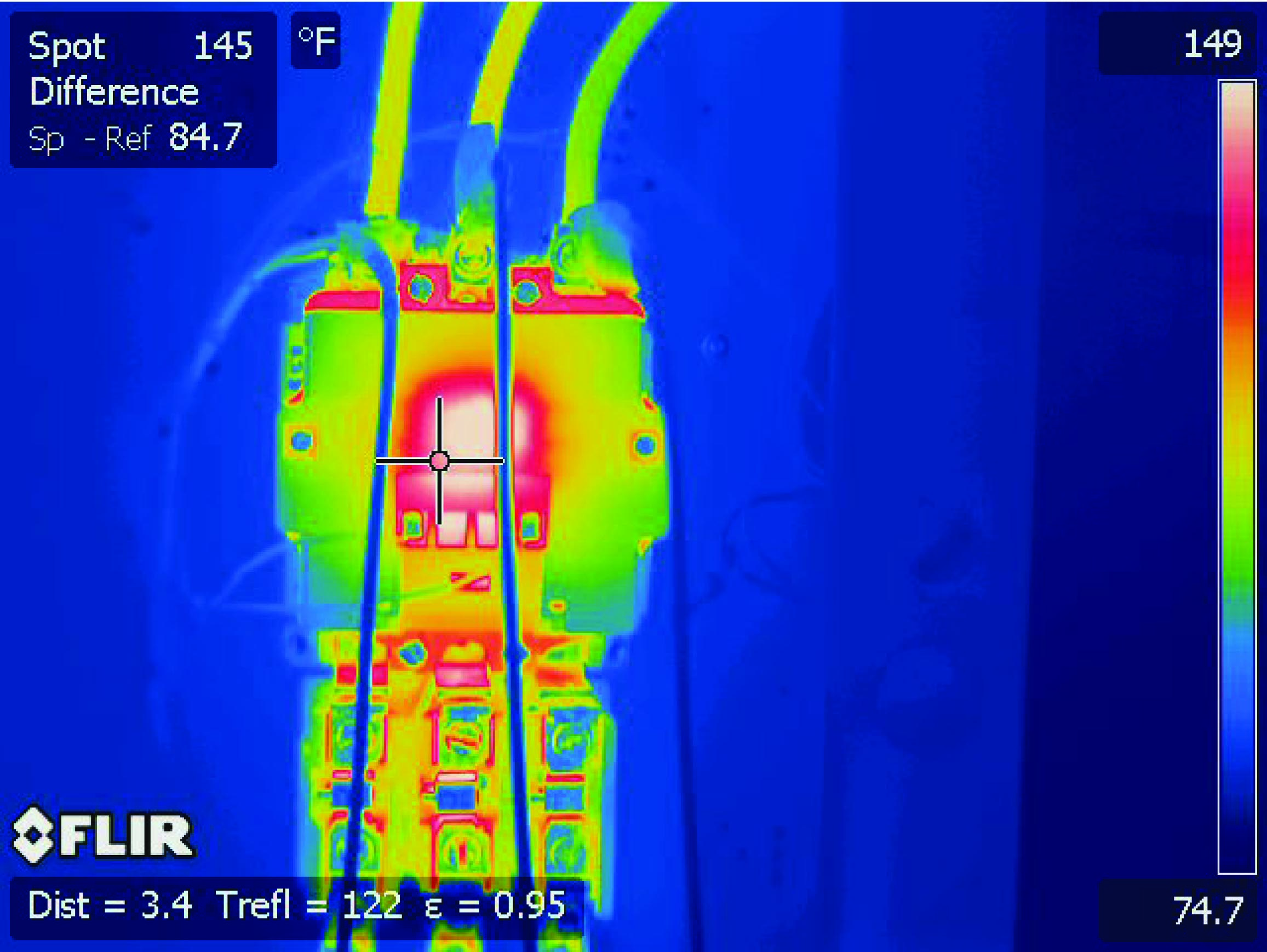
The bright spot in the center of the contactor is the higher temperature of the electromagnetic coil, providing magnetic force to actuate the contactor mechanism. Perhaps the most telling detail of this thermal image, however, is the difference in temperature between the overload heater connections (the six screws located near the bottom of the starter assembly). Note how the middle heater’s screws register slightly higher temperatures than the screws on either of the other two heater elements. Large temperature differences may indicate poor electrical connections (i.e. greater resistance) at the hot spots, or imbalances in phase current. It is also possible that the elevated temperature of this particular overload heater is simply due to it having less open surface area for it to radiate heat, since the two overload heaters flanking it enjoy the advantage of having more air cooling. If three people pack themselves into a narrow bench seat, the middle person is going to be warmer than either of the outer two!
Another noteworthy detail in this image is the “Spot Difference” measurement provided by the thermal imager. A cross-hair cursor on the display serves to locate a particular spot in the image, which in this case is contrasted against a reference spot chosen in an earlier step. The instrument automatically subtracts the current and reference spot temperatures to give a \(\Delta T\) indication, in this particular case 84.7 \(^{o}\)F.
A thermal image of a three-phase circuit breaker shows a much more even distribution of temperature:
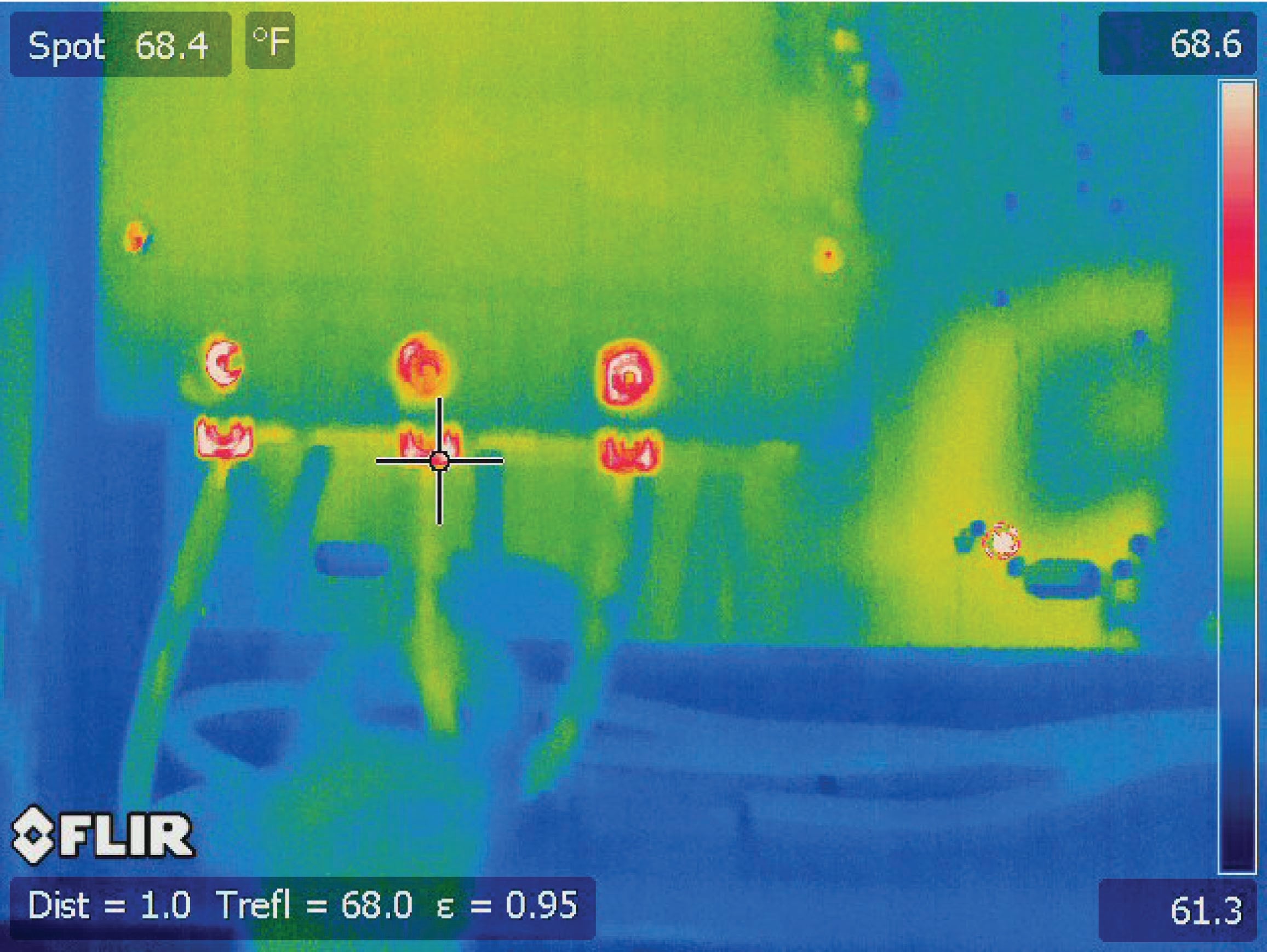
The hottest objects in this image are the three load screw terminals, appearing as white/red against a blue/green background. Note the range of the temperature scale on the right of the image: this particular image only spans a temperature range of 61.3 \(^{o}\)F to 68.6 \(^{o}\)F. This narrow temperature range tells us the differences in temperature shown by colors in this image are nothing to worry about.
Here, the instrument provides a single-point temperature measurement of 68.4 \(^{o}\)F at the cursor (“Spot”) location rather than a differential temperature measurement between two points.
