 Facebook
 Google
 GitHub
 Linkedin
Standardized Volumetric Flow
The majority of flowmeter technologies operate on the principle of interpreting fluid flow based on the velocity of the fluid. Magnetic, ultrasonic, turbine, and vortex flowmeters are prime examples, where the sensing elements (of each meter type) respond directly to fluid velocity. Translating fluid velocity into volumetric flow is quite simple, following this equation:
\[Q = A \overline{v}\]
Where,
\(Q\) = Volumetric flow rate (e.g. cubic feet per minute)
\(A\) = Cross-sectional area of flowmeter throat (e.g. square feet)
\(\overline{v}\) = Average fluid velocity at throat section (e.g. feet per minute)
Positive displacement flowmeters are even more direct than velocity-sensing flowmeters. A positive displacement flowmeter directly measures volumetric flow, counting discrete volumes of fluid as it passes through the meter.
Even pressure-based flowmeters such as orifice plates and venturi tubes are usually calibrated to measure in units of volume over time (e.g. gallons per minute, barrels per hour, cubic feet per second, etc.). For a great many industrial fluid flow applications, measurement in volumetric units makes sense.
This is especially true if the fluid in question is a liquid. Liquids are essentially incompressible: that is, they do not easily yield in volume to applied pressure. This makes volumetric flow measurement relatively simple for liquids: one cubic foot of a liquid at high pressure inside a process vessel will occupy approximately the same volume (\(\approx\) 1 ft\(^{3}\)) when stored in a barrel at atmospheric pressure.
Gases and vapors, however, easily change volume under the influences of both pressure and temperature. In other words, a gas will yield to an increasing pressure by decreasing in volume as the gas molecules are forced closer together, and it will yield to a decreasing temperature by decreasing in volume as the kinetic energy of the individual molecules is reduced. This makes volumetric flow measurement more complex for gases than for liquids. One cubic foot of gas at high pressure and temperature inside a process vessel will not occupy one cubic foot under ambient pressure and temperature conditions.
The practical difference between volumetric flow measurement for liquids versus gases is easily seen through an example where we measure the volumetric flow rate before and after a pressure-reduction valve:
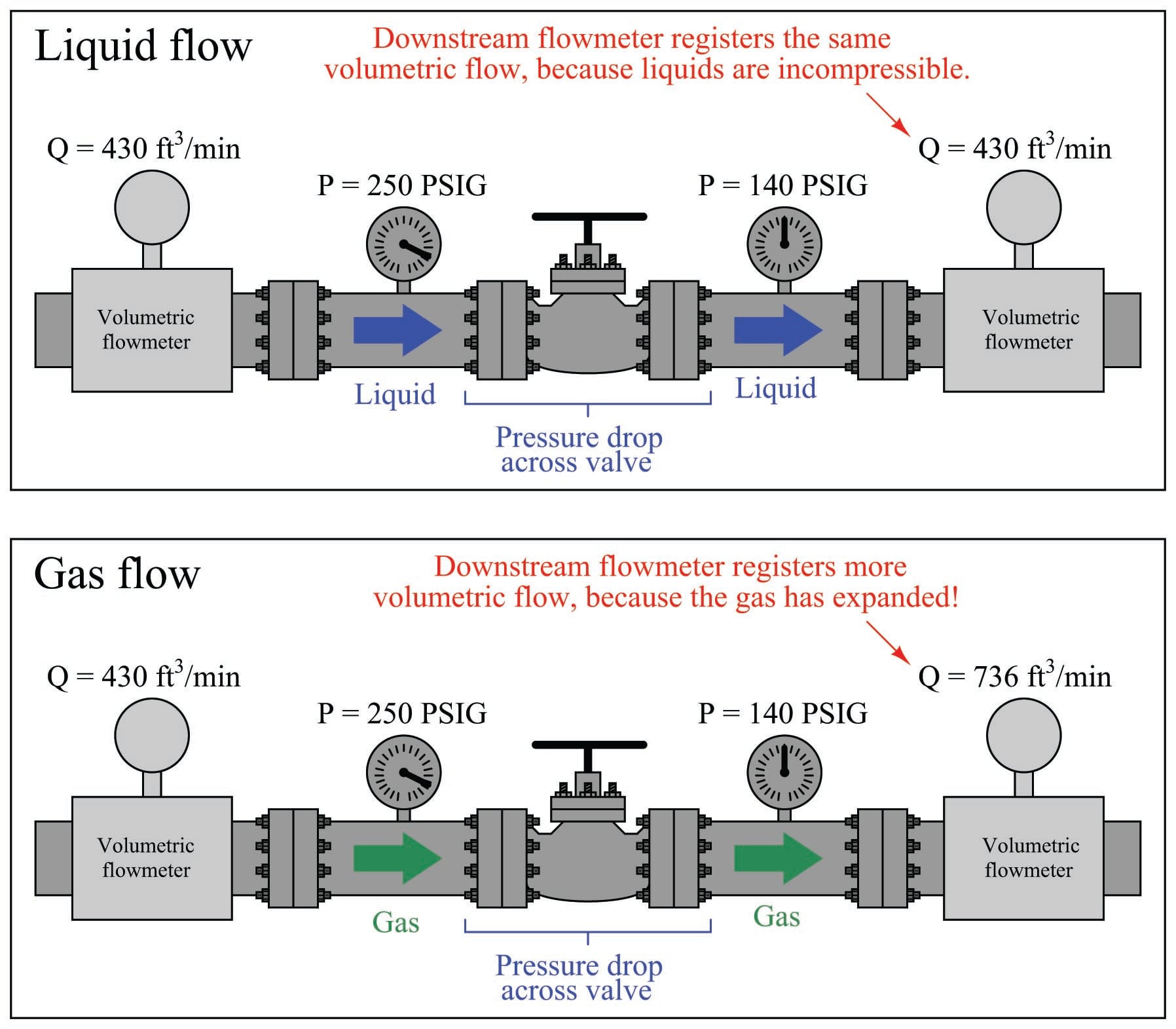
The volumetric flow rate of liquid before and after the pressure-reducing valve is the same, since the volume of a liquid does not depend on the pressure applied to it (i.e. liquids are incompressible). The volumetric flow rate of the gas, however, is significantly greater following the pressure-reducing valve than before, since the reduction in pressure allows the gas to expand (i.e. less pressure means the gas occupies a greater volume).
What this tells us is that volumetric flow measurement for gas is virtually meaningless without accompanying data on pressure and temperature. A flow rate of “430 ft\(^{3}\)/min” reported by a flowmeter measuring gas at 250 PSIG means something completely different than the same volumetric flow rate (430 ft\(^{3}\)/min) reported at a different line pressure.
One solution to this problem is to dispense with volumetric flow measurement altogether in favor of mass flow measurement, constructing the flowmeter in such a way that the actual mass of the gas molecules is measured as they pass through the instrument. This approach is explored in more detail in section 22.7 beginning on page . A more traditional approach to this problem is to specify gas flow in volume units per time, at some agreed-upon (standardized) set of pressure and temperature conditions. This is known as standardized volumetric flow measurement.
Referring to our pictorial example previously shown, imagine if we took a sample of the gas flowing at a line pressure of 250 PSIG and let that sample expand to atmospheric pressure (0 PSIG), measuring its new volume under those new conditions. For the sake of keeping this example simple, we will consider only a change in pressure, but not a change in temperature. Obviously, one cubic foot of gas at 250 PSIG would expand to a far greater volume than 1 ft\(^{3}\) at atmospheric pressure. This ratio of “standard volume” to “actual volume” (in the pressurized pipe) could then be used to scale the flowmeter’s measurement, so that the flowmeter registers in standard cubic feet per minute, or SCFM:
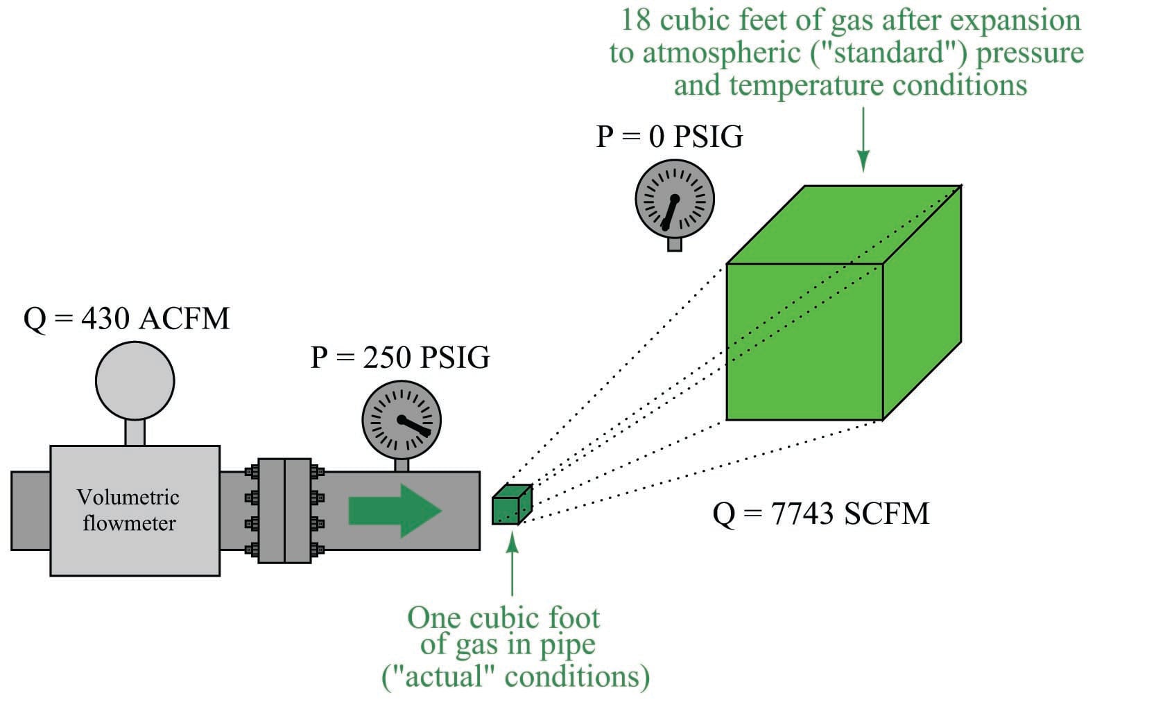
Assuming the same temperature inside the pipe as outside, the expansion ratio for this gas will be approximately 18:1, meaning the “actual” flowing rate of 430 ft\(^{3}\)/min is equivalent to approximately 7743 ft\(^{3}\)/min of gas flow at “standard” atmospheric conditions. In order to unambiguously distinguish “actual” volumetric flow rate from “standardized” volumetric flow rate, we commonly preface each unit with a letter “A” or letter “S” (e.g. ACFM and SCFM).
If a volumetric-registering flowmeter is equipped with pressure and temperature sensors, it may automatically scale its own output signal to measure gas flow rate in standard volumetric units. All we need to determine is the mathematical procedure to scale actual conditions to standard conditions for a gas. To do this, we will refer to the Ideal Gas Law (\(PV = nRT\)), which is a fair approximation for most real gases at conditions far from their critical phase-change points. First, we shall write two versions of the Ideal Gas Law, one for the gas under “standard” atmospheric conditions, and one for the gas under “actual” flowing conditions (using the subscripts “S” and “A” to distinguish one set of variables from the other):
\[P_S V_S = nR T_S\]
\[P_A V_A = nR T_A\]
What we need to do is determine the ratio of standard volume to actual volume (\(V_S \over V_A\)). To do this, we may divide one equation by the other:
\[{P_S V_S \over P_A V_A} = {nR T_S \over nR T_A}\]
Seeing that both the \(n\) variables are identical and \(R\) is a constant, we may cancel them both from the right-hand side of the equation:
\[{P_S V_S \over P_A V_A} = {T_S \over T_A}\]
Solving for the ratio \(V_S \over V_A\):
\[{V_S \over V_A} = {P_A T_S \over P_S T_A}\]
Since we know the definition of volumetric flow (\(Q\)) is volume over time (\(V \over t\)), we may divide each \(V\) variable by \(t\) to convert this into a volumetric flow rate correction ratio:
\[{{V_S \over t} \over {V_A \over t}} = {P_A T_S \over P_S T_A}\]
This leaves us with a ratio of “standardized” volumetric flow (\(Q_S\)) to “actual” volumetric flow (\(Q_A\)), for any known pressures and temperatures, standard to actual:
\[{Q_S \over Q_A} = {P_A T_S \over P_S T_A}\]
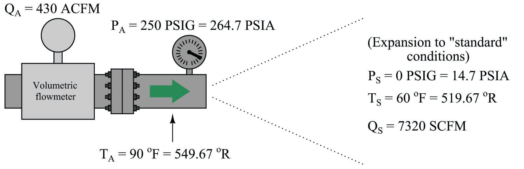
We may apply this to a practical example, assuming flowing conditions of 250 PSIG and 90 degrees Fahrenheit, and “standard” conditions of 0 PSIG and 60 degrees Fahrenheit. It is very important to ensure all values for pressure and temperature are expressed in absolute units (e.g. PSIA and degrees Rankine), which is what the Ideal Gas Law assumes:
\[{Q_S \over Q_A} = {P_A T_S \over P_S T_A}\]
\[Q_S = Q_A \left({P_A T_S \over P_S T_A}\right)\]
\[7320 \hbox{ SCFM} = (430 \hbox{ ACFM}) \left({(264.7 \hbox{ PSIA}) (519.67^{o}\hbox{R}) \over (14.7 \hbox{ PSIA}) (549.67^o \hbox{R})}\right)\]
This figure of 7320 SCFM indicates the volumetric flow rate of the gas through the pipe had it been allowed to expand to atmospheric pressure and cool to ambient temperature. Although we know these are definitely not the same conditions inside the gas pipe, the correction of actual volumetric flow measurement to these imagined conditions allows us to express gas flow rates in an equitable fashion regardless of the process line pressure or temperature. To phrase this in colloquial terms, standardized volumetric flow figures allow us to compare different process gas flow rates on an “apples to apples” basis, instead of the “apples to oranges” problem we faced earlier where flowmeters would register different volumetric flow values because their line pressures and/or flowing temperatures differed.
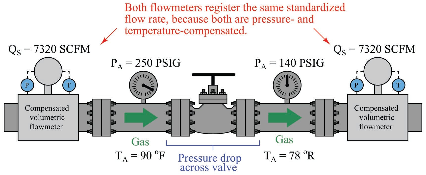
With pressure and temperature compensation integrated into volumetric flowmeters, we should be able to measure the exact same standardized flow rate at any point in a series gas piping system regardless of pressure or temperature changes:
An unfortunate state of affairs is the existence of multiple “standard” conditions of pressure and temperature defined by different organizations. In the previous example, 14.7 PSIA was assumed to be the “standard” atmospheric pressure, and 60 degrees Fahrenheit (519.67 degrees Rankine) was assumed to be the “standard” ambient temperature. This conforms to the API (American Petroleum Institute) standards in the United States of America, but it does not conform to other standards in America or in Europe. The ASME (American Society of Mechanical Engineers) uses 14.7 PSIA and 68 degrees Fahrenheit (527.67 degrees Rankine) as their “standard” conditions for calculating SCFM. In Europe, the PNEUROP agency has standardized with the American CAGI (Compressed Air and Gas Institute) organization on 14.5 PSIA and 68 degrees Fahrenheit being the “standard” conditions.
For gas flows containing condensible vapors, the partial pressures of the vapors must be subtracted from the absolute pressures (\(P_A\) and \(P_S\)) in order that the correction factor accurately reflects gas behavior alone. A common application of standardized gas flow involving partial pressure correction is found in compressed air systems, where water vapor (relative humidity) is a factor. Here too, standards differ as to the humidity conditions of “standard” cubic feet. The API and PNEUROP/CAGI standards call for 0% humidity (perfectly dry air) as the “standard,” while the ASME defines 35% relative humidity as “standard” for compressed air calculations.
