 Facebook
 Google
 GitHub
 Linkedin
Velocity-based Flowmeters
The Law of Continuity for fluids states that the product of mass density (\(\rho\)), cross-sectional pipe area (\(A\)) and average velocity (\(\overline{v}\)) must remain constant through any continuous length of pipe:
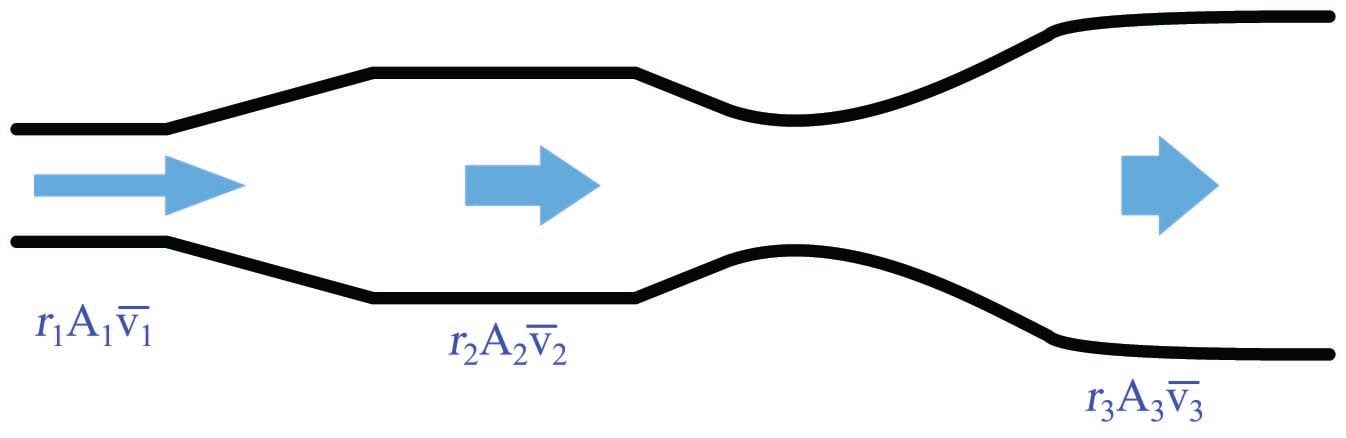
If the density of the fluid is not subject to change as it travels through the pipe (a very good assumption for liquids), we may simplify the Law of Continuity by eliminating the density terms from the equation:
\[A_1 \overline{v_1} = A_2 \overline{v_2}\]
The product of cross-sectional pipe area and average fluid velocity is the volumetric flow rate of the fluid through the pipe (\(Q = A\overline{v}\)). This tells us that fluid velocity will be directly proportional to volumetric flow rate given a known cross-sectional area and a constant density for the fluid flowstream. Any device able to directly measure fluid velocity is therefore capable of inferring volumetric flow rate of fluid in a pipe. This is the basis for velocity-based flowmeter designs.
Turbine flowmeters
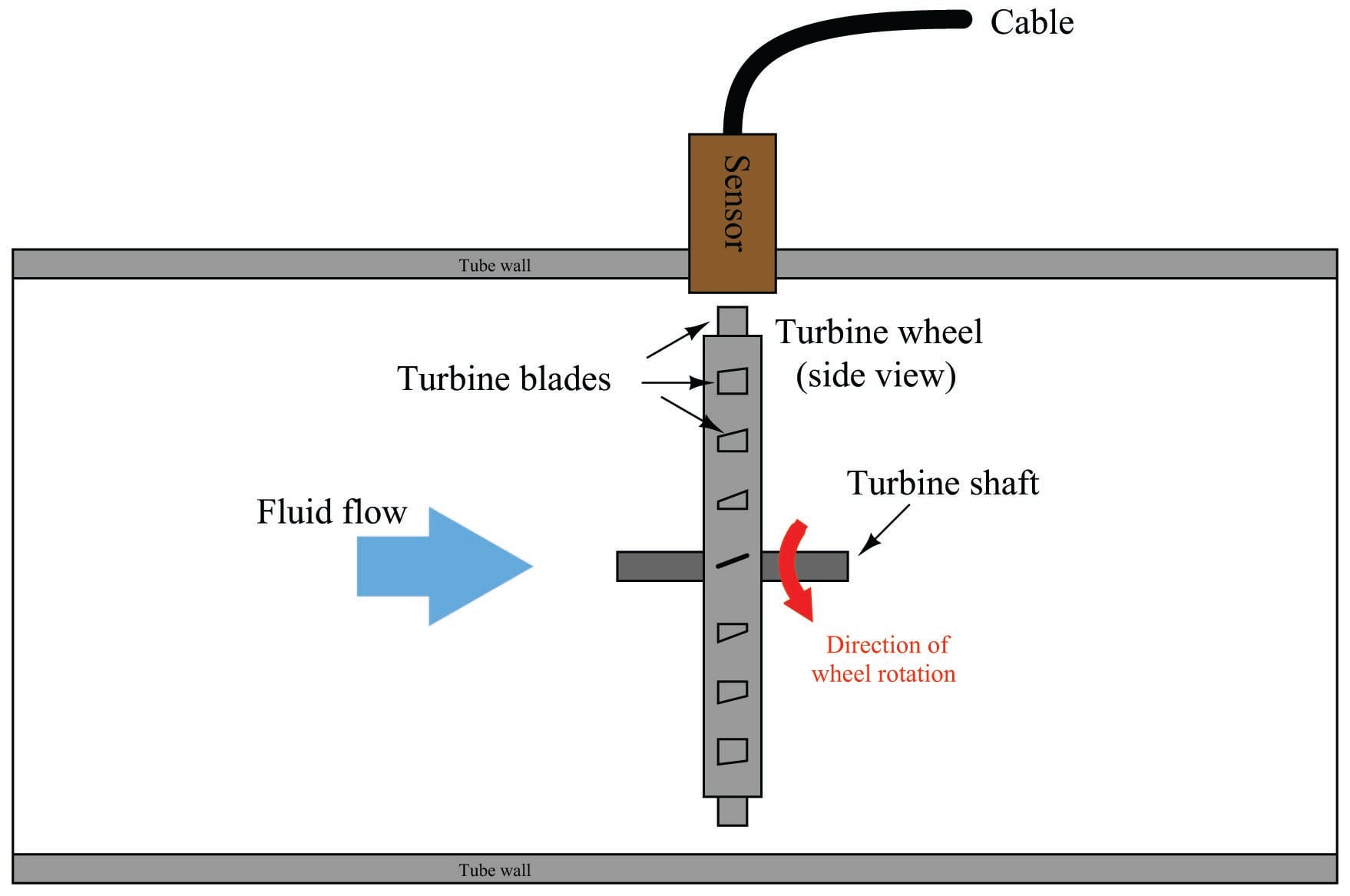
Turbine flowmeters use a free-spinning turbine wheel to measure fluid velocity, much like a miniature windmill installed in the flow stream. The fundamental design goal of a turbine flowmeter is to make the turbine element as free-spinning as possible, so no torque will be required to sustain the turbine’s rotation. If this goal is achieved, the turbine blades will achieve a rotating (tip) velocity directly proportional to the linear velocity of the fluid, whether that fluid is a gas or a liquid:
The mathematical relationship between fluid velocity and turbine tip velocity – assuming frictionless conditions – is a ratio defined by the tangent of the turbine blade angle:
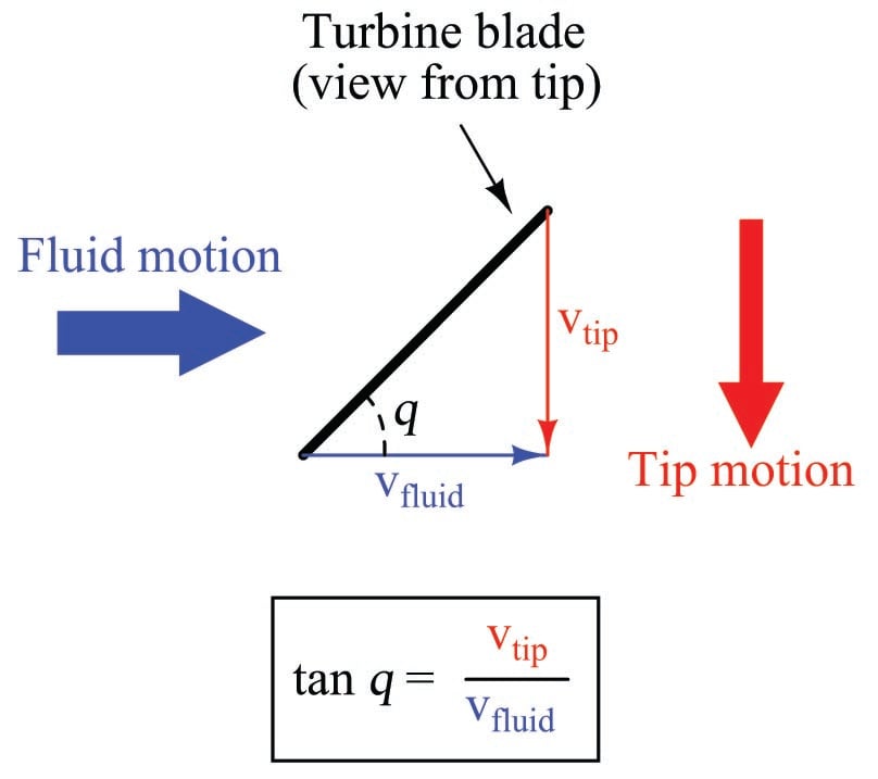
For a 45\(^{o}\) blade angle, the relationship is 1:1, with tip velocity equaling fluid velocity. Smaller blade angles (each blade closer to parallel with the fluid velocity vector) result in the tip velocity being a fractional proportion of fluid velocity.
Turbine tip velocity is quite easy to sense using a magnetic sensor, generating a voltage pulse each time one of the ferromagnetic turbine blades passes by. Traditionally, this sensor is nothing more than a coil of wire in proximity to a stationary magnet, called a pickup coil or pickoff coil because it “picks” (senses) the passing of the turbine blades. Magnetic flux through the coil’s center increases and decreases as the passing of the steel turbine blades presents a varying reluctance (“resistance” to magnetic flux), causing voltage pulses equal in frequency to the number of blades passing by each second. It is the frequency of this signal that represents fluid velocity, and therefore volumetric flow rate.
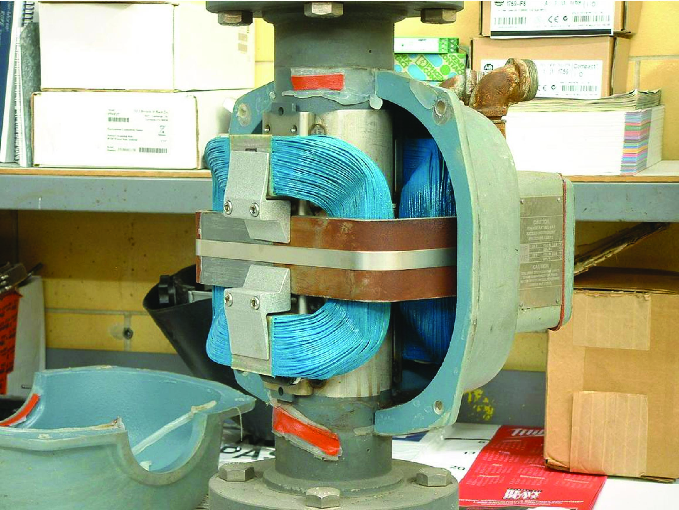
A cut-away demonstration model of a turbine flowmeter is shown in the following photograph. The blade sensor may be seen protruding from the top of the flowtube, just above the turbine wheel:
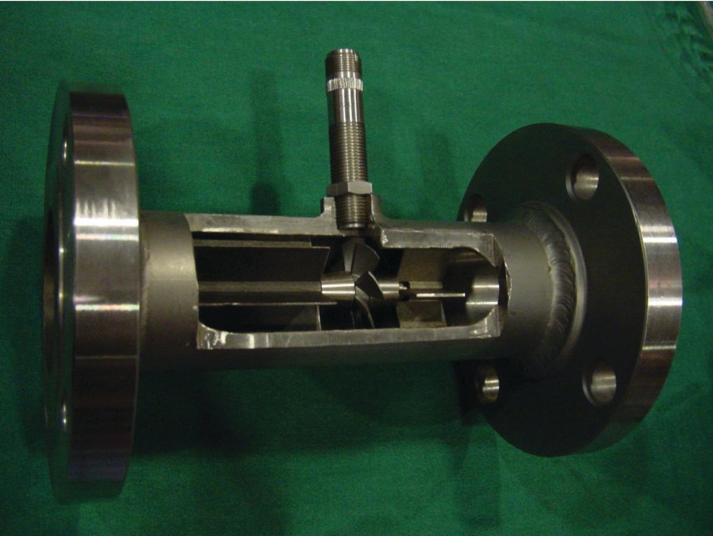
Note the sets of “flow conditioner” vanes immediately before and after the turbine wheel in the photograph. As one might expect, turbine flowmeters are very sensitive to swirl in the process fluid flowstream. In order to achieve high accuracy, the flow profile must not be swirling in the vicinity of the turbine, lest the turbine wheel spin faster or slower than it should to represent the velocity of a straight-flowing fluid. A minimum straight-pipe length of 20 pipe diameters upstream and 5 pipe diameters downstream is typical for turbine flowmeters in order to dissipate swirl from piping disturbances.
Mechanical gears and rotating cables have also been historically used to link a turbine flowmeter’s turbine wheel to indicators. These designs suffer from greater friction than electronic (“pickup coil”) designs, potentially resulting in more measurement error (less flow indicated than there actually is, because the turbine wheel is slowed by friction). One advantage of mechanical turbine flowmeters, though, is the ability to maintain a running total of gas usage by turning a simple odometer-style totalizer. This design is often used when the purpose of the flowmeter is to track total fuel gas consumption (e.g. natural gas used by a commercial or industrial facility) for billing.
In an electronic turbine flowmeter, volumetric flow is directly and linearly proportional to pickup coil output frequency. We may express this relationship in the form of an equation:
\[f = kQ\]
Where,
\(f\) = Frequency of output signal (Hz, equivalent to pulses per second)
\(Q\) = Volumetric flow rate (e.g. gallons per second)
\(k\) = “K” factor of the turbine element (e.g. pulses per gallon)
Dimensional analysis confirms the validity of this equation. Using units of GPS (gallons per second) and pulses per gallon, we see that the product of these two quantities is indeed pulses per second (equivalent to cycles per second, or Hz):
\[\left[\hbox{Pulses} \over \hbox{s} \right] = \left[\hbox{Pulses} \over \hbox{gal} \right] \left[\hbox{gal} \over \hbox{s} \right]\]
Using algebra to solve for flow (\(Q\)), we see that it is the quotient of frequency and \(k\) factor that yields a volumetric flow rate for a turbine flowmeter:
\[Q = {f \over k}\]
The inherent linearity of a turbine flowmeter is a tremendous advantage over nonlinear flow elements such as venturi tubes and orifice plates because this linearity results in a much greater turndown ratio for accurate flow measurement. Contrasted against common orifice-type meters which are usually limited to turndown ratios of 4:1 at best, turbine meters commonly exceed turndown ratios of 10:1.
If pickup signal frequency directly represents volumetric flow rate, then the total number of pulses accumulated in any given time span will represent the amount of fluid volume (\(V\)) passed through the turbine meter over that same time span. We may express this algebraically as the product of average flow rate (\(\overline{Q}\)), average frequency (\(\overline{f}\)), \(k\) factor, and time:
\[V = \overline{Q}t = {\overline{f} t \over k}\]
A more sophisticated way of calculating total volume passed through a turbine meter requires calculus, representing change in volume as the time-integral of instantaneous signal frequency and \(k\) factor over a period of time from \(t = 0\) to \(t = T\):
\[\Delta V = \int^T_0 Q \> dt \hbox{\hskip 30pt or \hskip 30pt} \Delta V = \int^T_0 {f \over k} \> dt\]
We may achieve approximately the same result simply by using a digital counter circuit to totalize pulses output by the pickup coil and a microprocessor to calculate volume in whatever unit of measurement we deem appropriate.
As with the orifice plate flow element, standards have been drafted for the use of turbine flowmeters as precision measuring instruments in gas flow applications, particularly the custody transfer of natural gas. The American Gas Association has published a standard called the Report #7 specifying the installation of turbine flowmeters for high-accuracy gas flow measurement, along with the associated mathematics for precisely calculating flow rate based on turbine speed, gas pressure, and gas temperature.
Pressure and temperature compensation is relevant to turbine flowmeters in gas flow applications because the density of the gas is a strong function of both pressure and temperature. The turbine wheel itself only senses gas velocity, and so these other factors must be taken into consideration to accurately calculate mass flow (or standard volumetric flow; e.g. SCFM).
In high-accuracy applications, it is important to individually determine the \(k\) factor for a turbine flowmeter’s calibration. Manufacturing variations from flowmeter to flowmeter make precise duplication of \(k\) factor challenging, and so a flowmeter destined for high-accuracy measurement should be tested against a “flow prover” in a calibration laboratory to empirically determine its \(k\) factor. If possible, the best way to test the flowmeter’s \(k\) factor is to connect the prover to the meter on site where it will be used. This way, the any effects due to the piping before and after the flowmeter will be incorporated in the measured \(k\) factor.
The following photograph shows three AGA7-compliant installations of turbine flowmeters for measuring the flow rate of natural gas:
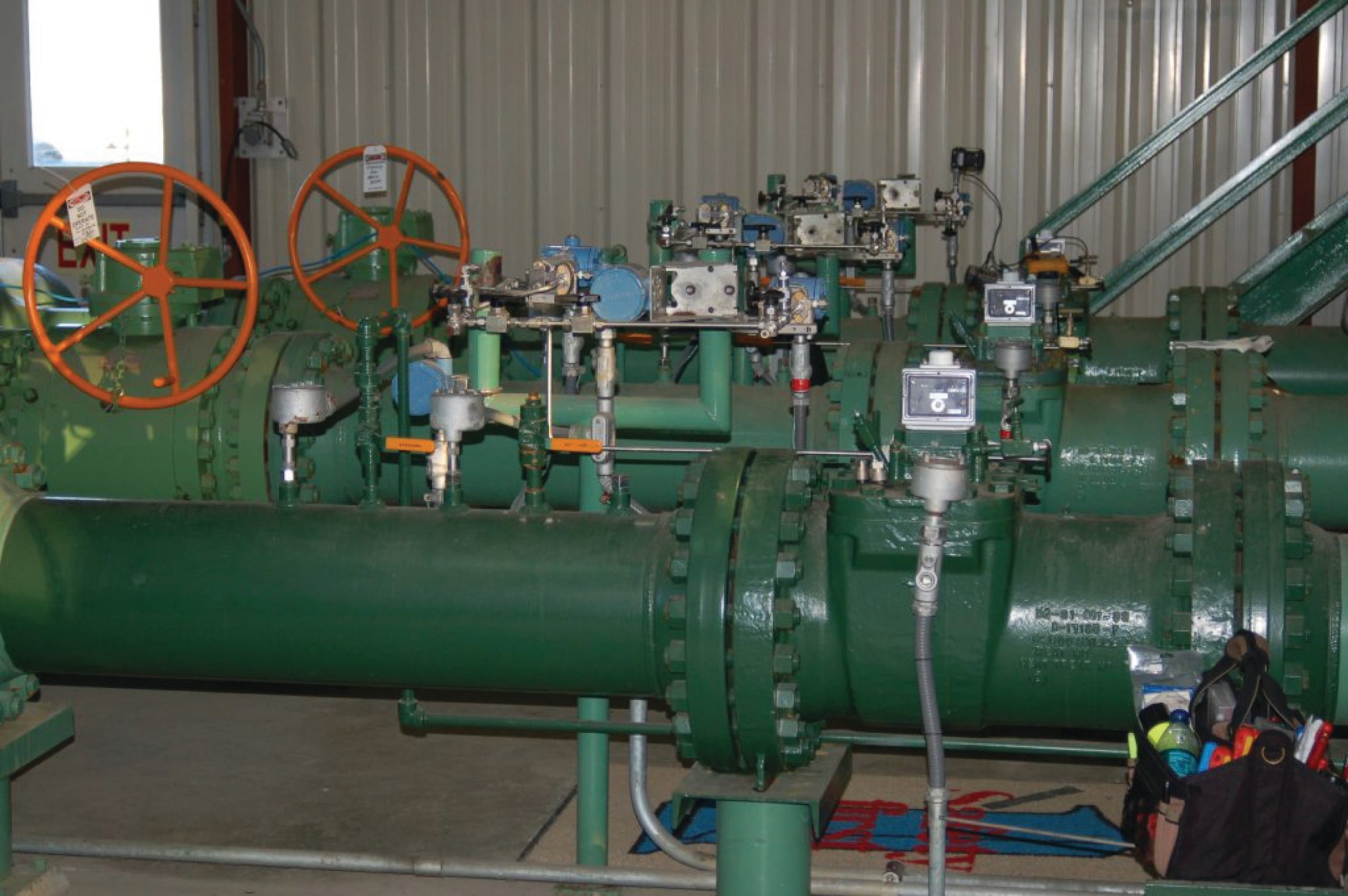
Note the pressure-sensing and temperature-sensing instrumentation installed in the pipe, reporting gas pressure and gas temperature to a flow-calculating computer (along with turbine pulse frequency) for the calculation of natural gas flow rate.
Less-critical gas flow measurement applications may use a “compensated” turbine flowmeter that mechanically performs the same pressure- and temperature-compensation functions on turbine speed to achieve true gas flow measurement, as shown in the following photograph:
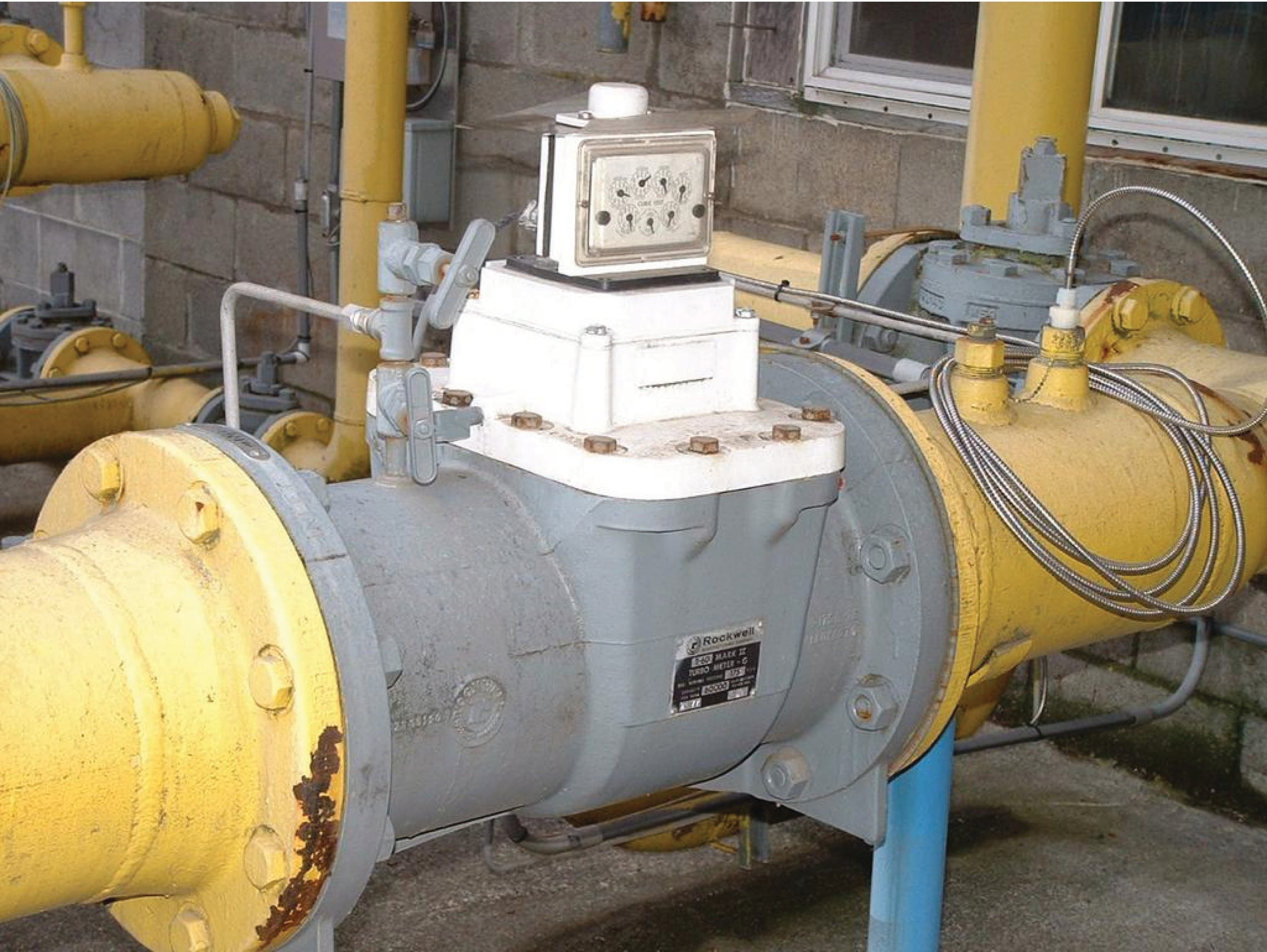
The particular flowmeter shown in the above photograph uses a filled-bulb temperature sensor (note the coiled, armored capillary tube connecting the flowmeter to the bulb) and shows total gas flow by a series of pointers, rather than gas flow rate.
A variation on the theme of turbine flow measurement is the paddlewheel flowmeter, a very inexpensive technology usually implemented in the form of an insertion-type sensor. In this instrument, a small wheel equipped with “paddles” parallel to the shaft is inserted in the flowstream, with half the wheel shrouded from the flow. A photograph of a plastic paddlewheel flowmeter appears here:
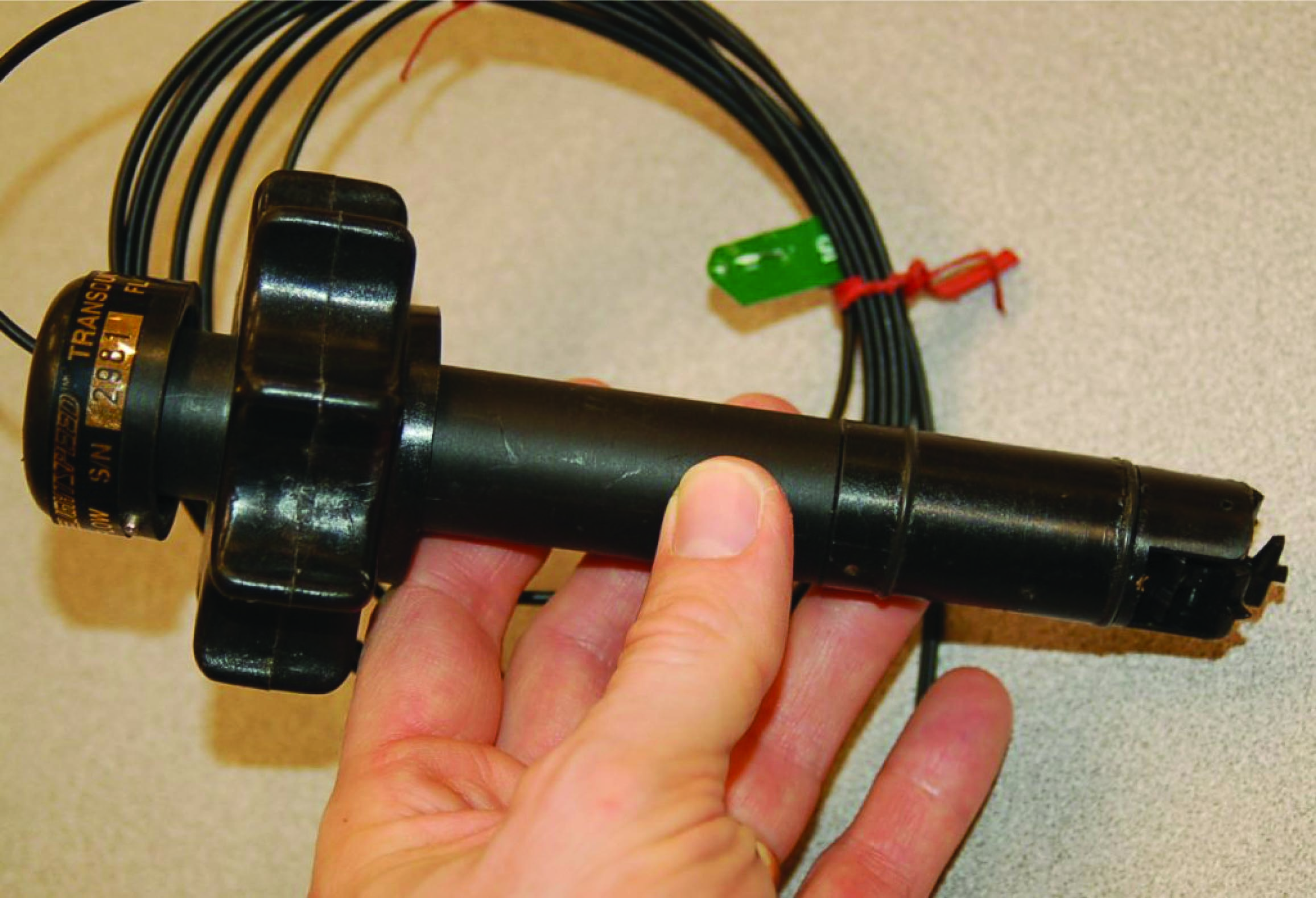
A surprisingly sophisticated method of “pickup” for the plastic paddlewheel shown in the photograph uses fiber-optic cables to send and receive light. One cable sends a beam of light to the edge of the paddlewheel, and the other cable receives light on the other side of the paddlewheel. As the paddlewheel turns, the paddles alternately block and pass the light beam, resulting in a pulsed light beam at the receiving cable. The frequency of this pulsing is, of course, directly proportional to volumetric flow rate.
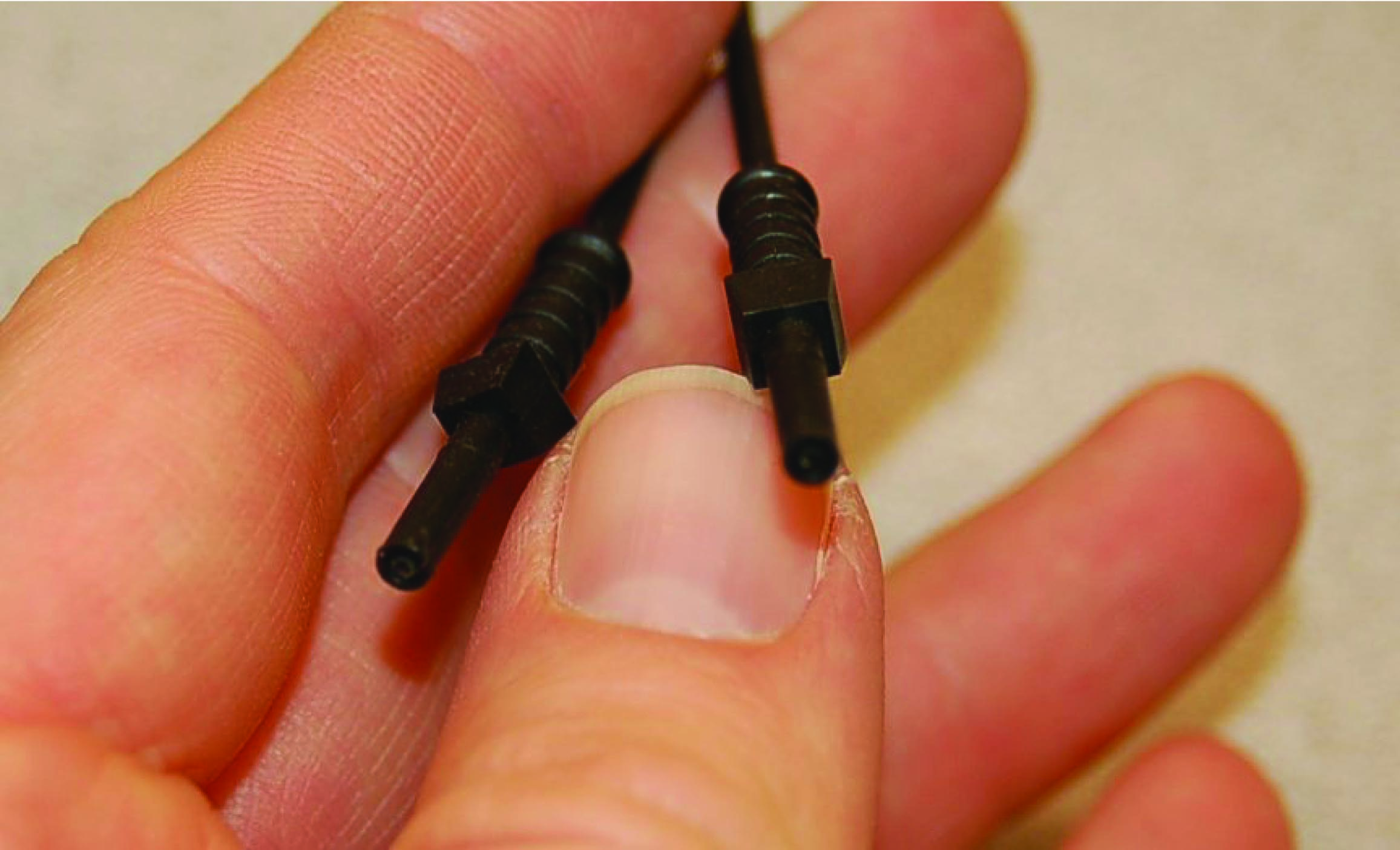
The external ends of the two fiber optic cables appear in this next photograph, ready to connect to a light source and light pulse sensor to convert the paddlewheel’s motion into an electronic signal:
A problem common to all turbine flowmeters is that of the turbine “coasting” when the fluid flow suddenly stops. This is more often a problem in batch processes than continuous processes, where the fluid flow is regularly turned on and shut off. This problem may be minimized by configuring the measurement system to ignore turbine flowmeter signals any time the automatic shutoff valve reaches the “shut” position. This way, when the shutoff valve closes and fluid flow immediately halts, any coasting of the turbine wheel will be irrelevant. In processes where the fluid flow happens to pulse for reasons other than the control system opening and shutting automatic valves, this problem is more severe.
Another problem common to all turbine flowmeters is lubrication of the turbine bearings. Frictionless motion of the turbine wheel is essential for accurate flow measurement, which is a daunting design goal for the flowmeter manufacturing engineers. The problem is not as severe in applications where the process fluid is naturally lubricating (e.g. diesel fuel), but in applications such as natural gas flow where the fluid provides no lubrication to the turbine bearings, external lubrication must be supplied. This is often a regular maintenance task for instrument technicians: using a hand pump to inject light-weight “turbine oil” into the bearing assemblies of turbine flowmeters used in gas service.
Process fluid viscosity is another source of friction for the turbine wheel. Fluids with high viscosity (e.g. heavy oils) will tend to slow down the turbine’s rotation even if the turbine rotates on frictionless bearings. This effect is especially pronounced at low flow rates, which leads to a minimum linear flow rating for the flowmeter: a flowrate below which it refuses to register proportionately to fluid flow rate.
Vortex flowmeters
When a fluid moves with high Reynolds number past a stationary object (a “bluff body”), there is a tendency for the fluid to form vortices on either side of the object. Each vortex will form, then detach from the object and continue to move with the flowing gas or liquid, one side at a time in alternating fashion. This phenomenon is known as vortex shedding, and the pattern of moving vortices carried downstream of the stationary object is known as a vortex street.
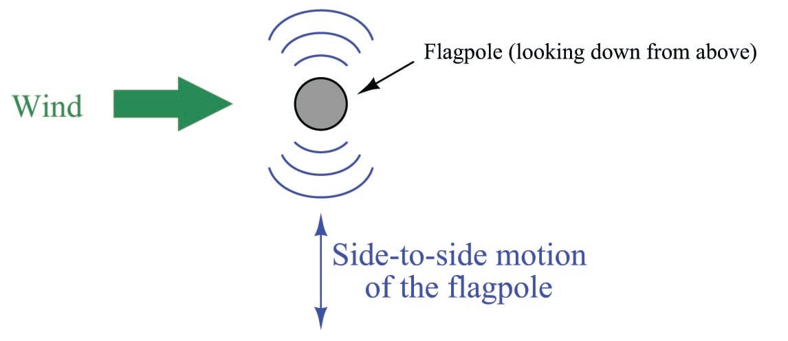
It is commonplace to see the effects of vortex shedding on a windy day by observing the motion of flagpoles, light poles, and tall smokestacks. Each of these objects has a tendency to oscillate perpendicular to the direction of the wind, owing to the pressure variations caused by the vortices as they alternately form and break away from the object:
This alternating series of vortices was studied by Vincenc Strouhal in the late nineteenth century and later by Theodore von Kármán in the early twentieth century. It was determined that the distance between successive vortices downstream of the stationary object is relatively constant, and directly proportional to the width of the object, for a wide range of Reynolds number values. If we view these vortices as crests of a continuous wave, the distance between vortices may be represented by the symbol customarily reserved for wavelength: the Greek letter “lambda” (\(\lambda\)).
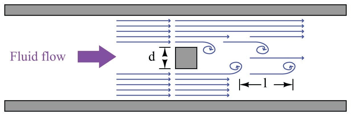
The proportionality between object width (\(d\)) and vortex street wavelength (\(\lambda\)) is called the Strouhal number (\(S\)), approximately equal to 0.17:
\[\lambda S = d \hbox{\hskip 50pt} \lambda \approx {d \over 0.17}\]
If a differential pressure sensor is installed immediately downstream of the stationary object in such an orientation that it detects the passing vortices as pressure variations, an alternating signal will be detected:
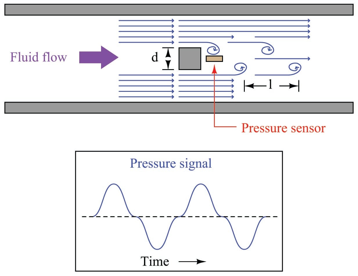
The frequency of this alternating pressure signal is directly proportional to fluid velocity past the object, since the wavelength is constant. This follows the classic frequency-velocity-wavelength formula common to all traveling waves (\(\lambda f = v\)). Since we know the wavelength will be equal to the bluff body’s width divided by the Strouhal number (approximately 0.17), we may substitute this into the frequency-velocity-wavelength formula to solve for fluid velocity (\(v\)) in terms of signal frequency (\(f\)) and bluff body width (\(d\)).
\[v = \lambda f\]
\[v = {d \over 0.17} f\]
\[v = {d f \over 0.17}\]
Thus, a stationary object and pressure sensor installed in the middle of a pipe section constitute a form of flowmeter called a vortex flowmeter. Like a turbine flowmeter with an electronic “pickup” sensor to detect the passage of rotating turbine blades, the output frequency of a vortex flowmeter is linearly proportional to volumetric flow rate.
The pressure sensors used in vortex flowmeters are not standard differential pressure transmitters, since the vortex frequency is too high to be successfully detected by such bulky instruments. Instead, the sensors are typically piezoelectric crystals. These pressure sensors need not be calibrated, since the amplitude of the pressure waves detected is irrelevant. Only the frequency of the waves matter for measuring flow rate, and so nearly any pressure sensor with a fast enough response time will suffice.
Like turbine meters, the relationship between sensor frequency (\(f\)) and volumetric flow rate (\(Q\)) may be expressed as a proportionality, with the letter \(k\) used to represent the constant of proportionality for any particular flowmeter:
\[f = kQ\]
Where,
\(f\) = Frequency of output signal (Hz)
\(Q\) = Volumetric flow rate (e.g. gallons per second)
\(k\) = “K” factor of the vortex shedding flowtube (e.g. pulses per gallon)
This means vortex flowmeters, like electronic turbine meters, each have a particular “\(k\) factor” relating the number of pulses generated per unit volume passed through the meter. Counting the total number of pulses over a certain time span yields total fluid volume passed through the meter over that same time span, making the vortex flowmeter readily adaptable for “totalizing” fluid volume just like turbine meters. The direct proportion between vortex frequency and volumetric flow rate also means vortex flowmeters are linear-responding instruments just like turbine flowmeters. Unlike orifice plates which exhibit a quadratic response, turbine and vortex flowmeters alike enjoy a wider range (turndown) of flow measurement and do not require special signal characterization to function properly.
Since vortex flowmeters have no moving parts, they do not suffer the problems of wear and lubrication facing turbine meters. There is no moving element to “coast” as in a turbine flowmeter if fluid flow suddenly stops, which means vortex flowmeters are better suited to measuring erratic flows.
A significant disadvantage of vortex meters is a behavior known as low flow cutoff, where the flowmeter simply stops working below a certain flow rate. The reason for this is laminar flow: at low flow rates (i.e. low Reynolds number values) the effects of fluid viscosity overwhelm fluid momentum, preventing vortices from forming. This cessation of vortices causes the vortex flowmeter to register absolutely no flow at all even when there is still some (laminar) flow through the pipe. At high flow rates (i.e. high Reynolds number values), fluid momentum is enough to overcome viscosity and produce vortices, and the vortex flowmeter works just fine.
The phenomenon of low-flow cutoff for a vortex flowmeter at first seems analogous to the minimum linear flow limitation of a turbine flowmeter. However, vortex flowmeter low-flow cutoff is actually a far more severe problem. If the volumetric flow rate through a turbine flowmeter falls below the minimum linear value, the turbine continues to spin, albeit slower than it should. If the volumetric flow rate through a vortex flowmeter falls below the low-flow cutoff value, however, the flowmeter’s signal goes completely to zero, indicating no flow at all. This idiosyncrasy makes vortex flowmeters entirely unsuitable in applications where the desired flow measurement range extends all the way down to zero.
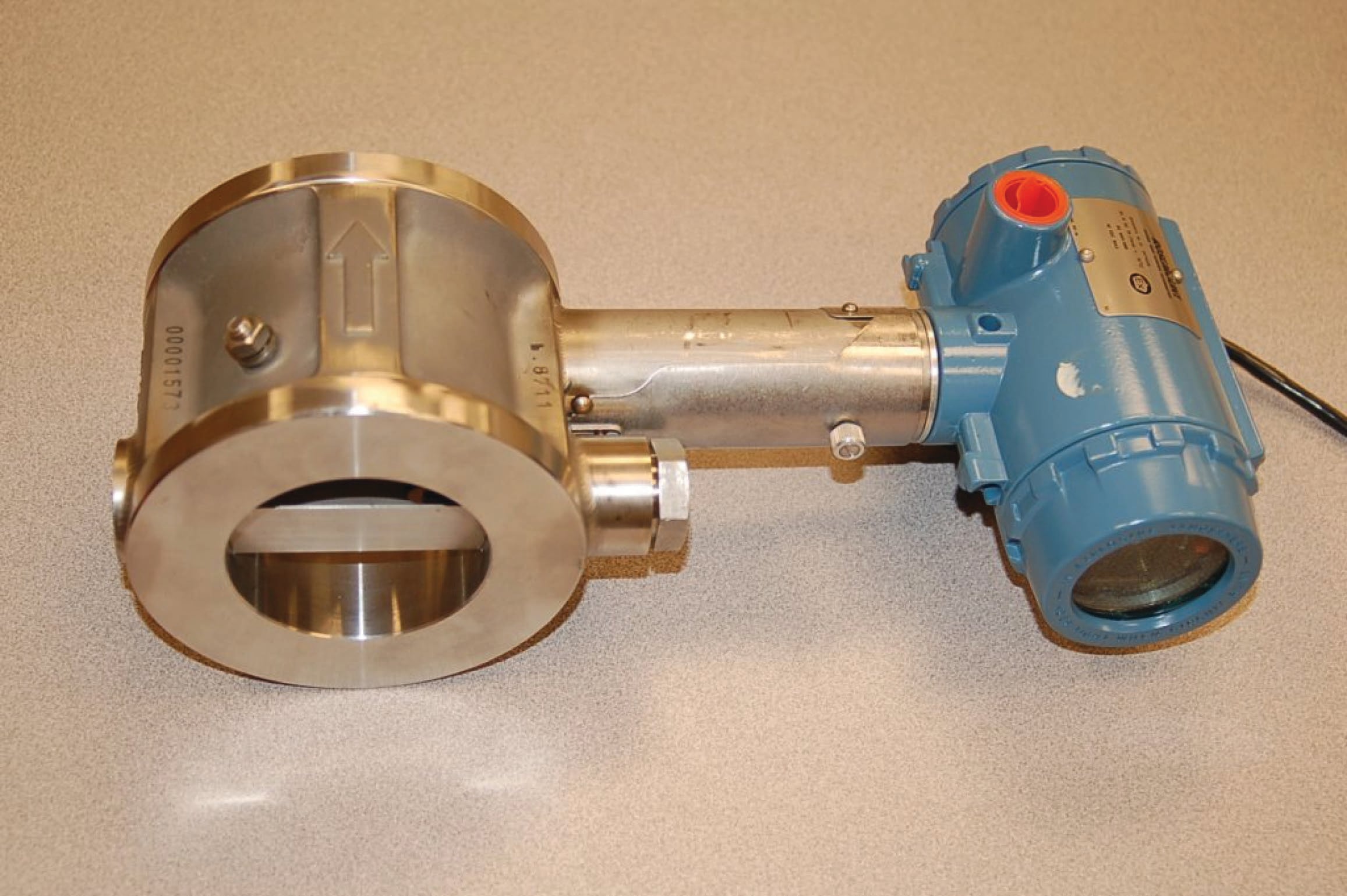
The following photograph shows a Rosemount model 8800C vortex flow transmitter:
The next two photographs show close-up views of the flowtube assembly, front (left) and rear (right):
Vortex flowmeters, like other velocity-based meters, are affected by large-scale turbulence in the fluid stream and therefore require some length of straight pipe both upstream and downstream of the flowmeter to properly characterize the flow. It is typical to install vortex flowmeters with 10 pipe diameters of straight-length pipe upstream and 5 pipe diameters downstream.
Magnetic flowmeters
When an electrical conductor moves perpendicular to a magnetic field, a voltage is induced in that conductor perpendicular to both the magnetic flux lines and the direction of motion. This phenomenon is known as electromagnetic induction, and it is the basic principle upon which all electro-mechanical generators operate.
In a generator mechanism, the conductor in question is typically a coil (or set of coils) made of copper wire. However, there is no reason the conductor must be made of copper wire. Any electrically conductive substance in motion is sufficient to electromagnetically induce a voltage, even if that substance is a liquid. Therefore, electromagnetic induction is a technique applicable to the measurement of liquid flow rates.
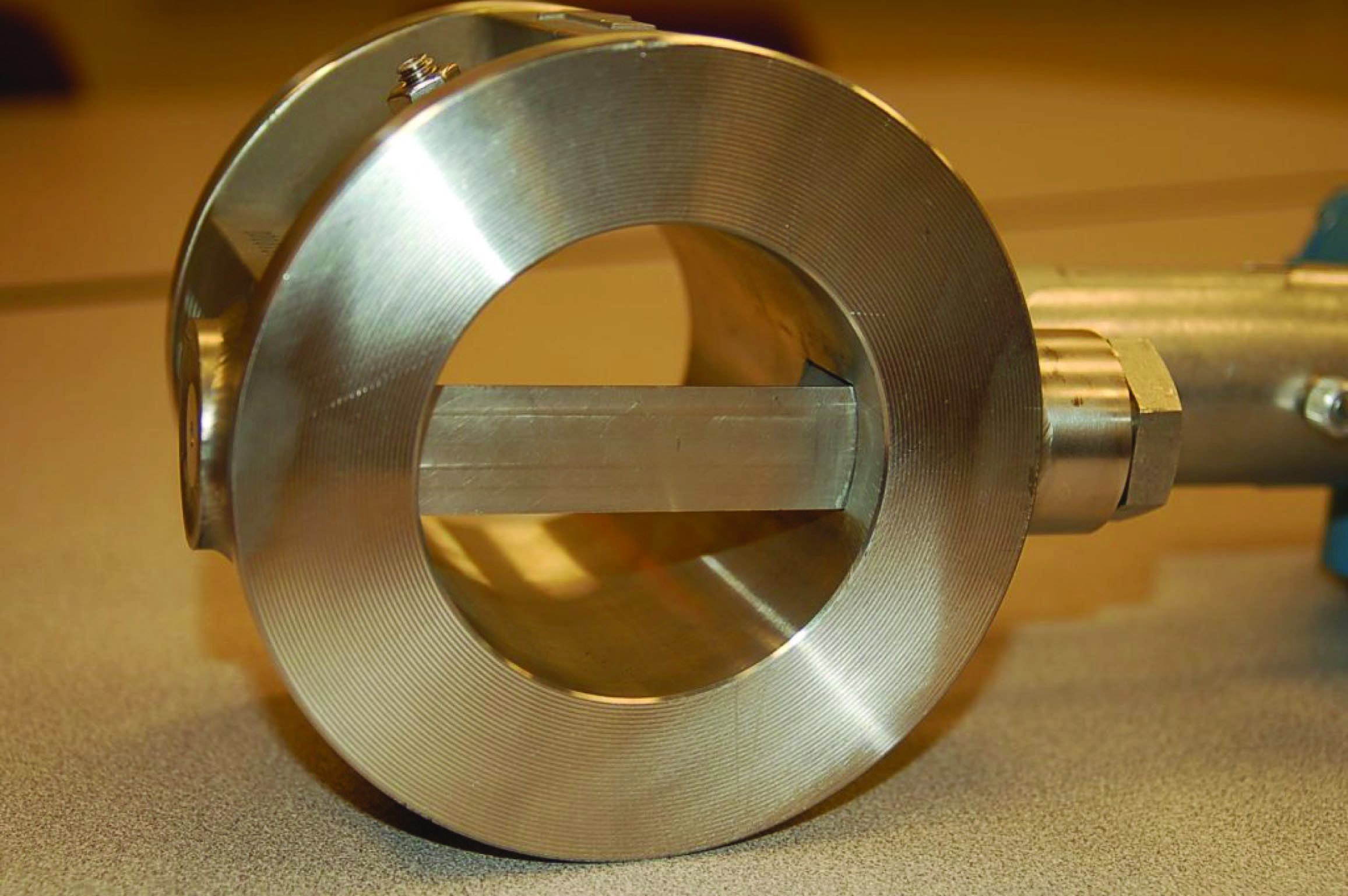
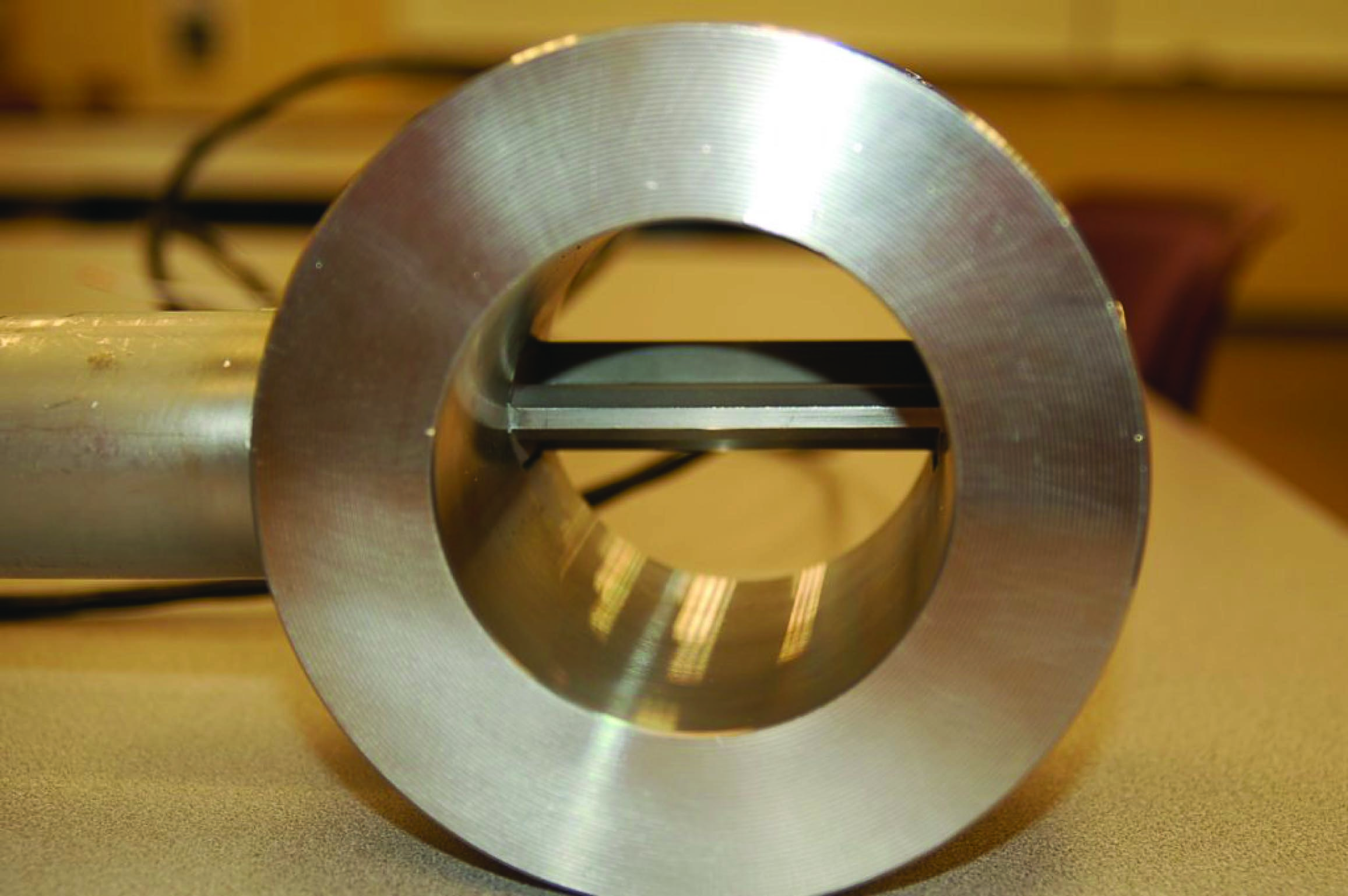
Consider water flowing through a pipe, with a magnetic field passing perpendicularly through the pipe:
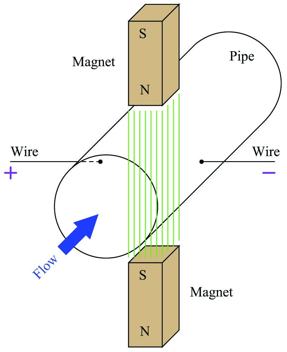
The direction of liquid flow cuts perpendicularly through the lines of magnetic flux, generating a voltage along an axis perpendicular to both. Metal electrodes opposite each other in the pipe wall intercept this voltage, making it readable to an electronic circuit.
A voltage induced by the linear motion of a conductor through a magnetic field is called motional EMF, the magnitude of which is predicted by the following formula (assuming perfect perpendicularity between the direction of velocity, the orientation of the magnetic flux lines, and the axis of voltage measurement):
\[\mathcal{E} = Blv\]
Where,
\(\mathcal{E}\) = Motional EMF (volts)
\(B\) = Magnetic flux density (Tesla)
\(l\) = Length of conductor passing through the magnetic field (meters)
\(v\) = Velocity of conductor (meters per second)
Assuming a fixed magnetic field strength (constant \(B\)) and an electrode spacing equal to the fixed diameter of the pipe (constant \(l = d\)), the only variable capable of influencing the magnitude of induced voltage is velocity (\(v\)). In our example, \(v\) is not the velocity of a wire segment, but rather the average velocity of the liquid flowstream (\(\overline{v}\)). Since we see that this voltage will be proportional to average fluid velocity, it must also be proportional to volumetric flow rate, since volumetric flow rate is also proportional to average fluid velocity. Thus, what we have here is a type of flowmeter based on electromagnetic induction. These flowmeters are commonly known as magnetic flowmeters or simply magflow meters.
We may state the relationship between volumetric flow rate (\(Q\)) and motional EMF (\(\mathcal{E}\)) more precisely by algebraic substitution. First, we will write the formula relating volumetric flow to average velocity, and then manipulate it to solve for average velocity:
\[Q = A\overline{v}\]
\[{Q \over A} = \overline{v}\]
Next, we re-state the motional EMF equation, and then substitute \(Q \over A\) for \(\overline{v}\) to arrive at an equation relating motional EMF to volumetric flow rate (\(Q\)), magnetic flux density (\(B\)), pipe diameter (\(d\)), and pipe area (\(A\)):
\[\mathcal{E} = Bd\overline{v}\]
\[\mathcal{E} = Bd {Q \over A}\]
\[\mathcal{E} = {BdQ \over A}\]
Since we know this is a circular pipe, we know that area and diameter are directly related to each other by the formula \(A = {\pi d^2 \over 4}\). Thus, we may substitute this definition for area into the last equation, to arrive at a formula with one less variable (only \(d\), instead of both \(d\) and \(A\)):
\[\mathcal{E} = {BdQ \over {\pi d^2 \over 4}}\]
\[\mathcal{E} = {BdQ \over 1} {4 \over {\pi d^2}}\]
\[\mathcal{E} = {4BQ \over {\pi d}}\]
If we wish to have a formula defining flow rate \(Q\) in terms of motional EMF (\(\mathcal{E}\)), we may simply manipulate the last equation to solve for \(Q\):
\[Q = {\pi d \mathcal{E} \over 4B}\]
This formula will successfully predict flow rate only for absolutely perfect circumstances. In order to compensate for inevitable imperfections, a “proportionality constant” (\(k\)) is usually included in the formula:
\[Q = k {\pi d \mathcal{E} \over 4B}\]
Where,
\(Q\) = Volumetric flow rate (cubic meters per second)
\(\mathcal{E}\) = Motional EMF (volts)
\(B\) = Magnetic flux density (Tesla)
\(d\) = Diameter of flowtube (meters)
\(k\) = Constant of proportionality
Note the linearity of this equation. Nowhere do we encounter a power, root, or other non-linear mathematical function in the equation for a magnetic flowmeter. This means no special characterization is required to calculate volumetric flow rate.
A few conditions must be met for this formula to successfully infer volumetric flow rate from induced voltage:
- The liquid must be a reasonably good conductor of electricity (note: it is okay if the conducting fluid contains some non-conducting solids; the conductive fluid surrounding the non-conducting solid matter still provides electrical continuity between the electrodes necessary for induction)
- The pipe must be completely filled with liquid to ensure contact with both probes as well as to ensure flow across the entire cross-section of the pipe
- The flowtube must be properly grounded to avoid errors caused by stray electric currents in the liquid
The first condition is met by careful consideration of the process liquid prior to installation. Magnetic flowmeter manufacturers will specify the minimum conductivity value of the liquid to be measured. The second and third conditions are met by correct installation of the magnetic flowtube in the pipe. The installation must be done in such a way as to guarantee full flooding of the flowtube (no gas pockets). The flowtube is usually installed with electrodes across from each other horizontally (never vertically!) so even a momentary gas bubble will not break electrical contact between an electrode tip and the liquid flowstream. The following photograph shows how not to install magnetic flowmeters:
Note in this example how the electrodes are vertically oriented instead of horizontal, because the pipes for these two magnetic flowmeters were placed too close to allow proper clearance for the protruding electrodes to lie horizontally. Sadly, poor flowmeter installation is all too common in new projects, as many piping designers and pipefitters are ignorant of flowmeter operating principles. This is one way instrument engineers and technicians may deter operational problems: by involving themselves in the design phase of a piping system, and helping to educate piping designers.
Magnetic flowmeters exhibit several advantages over other types of flowmeter. They are fairly tolerant of swirl and other large-scale turbulent fluid behavior, because the induced voltage is proportional only to the perpendicular velocity of the conductor, in this case the velocity of the fluid along the centerline of the flowtube. As such, magnetic flowmeters do not require the long straight-runs of pipe upstream and downstream that orifice plates do, which is a great advantage in many piping systems. Upstream straight-pipe requirements of 5 diameters and downstream straight-pipe requirements of 3 diameters is typical.
Additionally, the wide-open bore of a magnetic flowmeter’s tube means there is absolutely nothing to restrict the flow, resulting in extremely low permanent pressure loss. The lack of any obstruction within the path of fluid flow means magnetic flowmeters are quite tolerant of solids within the liquid flowstream, making them well-suited for measuring such process liquids as wastewater, slurries, wood pulp, and food products which might clog other types of flowmeters. In fact, magnetic flowmeters are the dominant flowmeter technology used in wastewater, wood pulping, and food processing industries for this very reason.
Electrical conductivity of the process liquid must meet a certain minimum value, but that is all. It is surprising to some technicians that changes in liquid conductivity have little to no effect on flow measurement accuracy. It is not as though a doubling of liquid conductivity will result in a doubling of induced voltage! Motional EMF is strictly a function of physical dimensions, magnetic field strength, and fluid velocity.
Liquids with poor conductivity present a greater electrical resistance in the voltage-measuring circuit than liquids with good conductivity, but this is of little consequence because the input impedance of the detection circuitry is phenomenally high. The effect of liquid conductivity on flowmeter operation may be modeled by the following DC circuits:
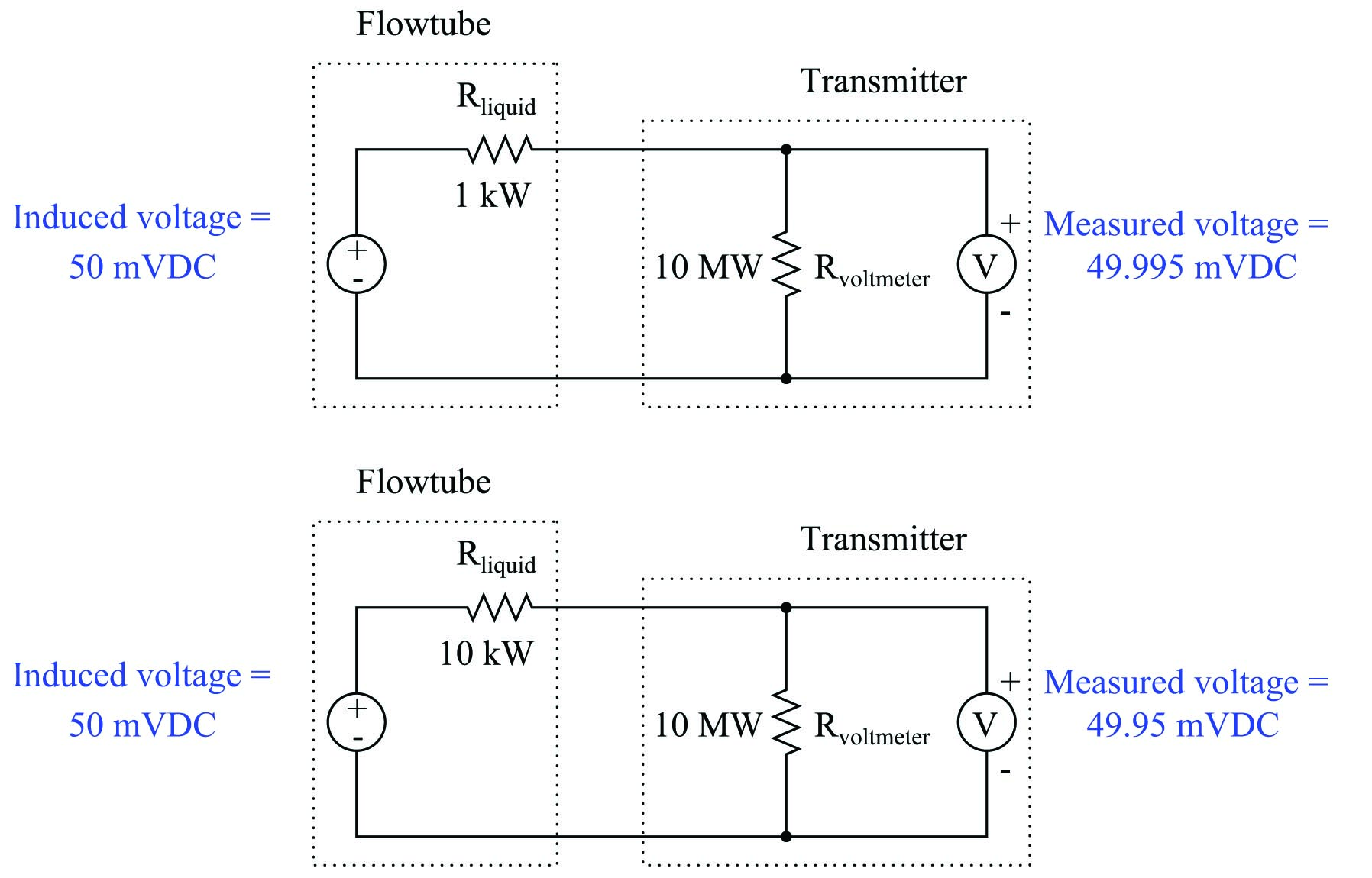
Here, a ten-fold (one order of magnitude) change in liquid resistance barely affects the measured voltage (49.995 mV versus 49.95 mV) because the flow transmitter’s voltage-sensing electronic circuit has such a high input impedance. The liquid’s equivalent resistance value must increase dramatically beyond the values shown in this example before it will have any significant effect on flow measurement accuracy.
In fact, the only time fluid conductivity is a problem with magnetic flowmeters is when the fluid in question has negligible conductivity. Such fluids include deionized water (e.g. steam boiler feedwater, ultrapure water for pharmaceutical and semiconductor manufacturing) and oils. Most aqueous (water-based) fluids work fine with magnetic flowmeters.
Proper grounding of the flowtube is very important for magnetic flowmeters. The motional EMF generated by most liquid flowstreams is very weak (1 millivolt or less!), and therefore may be easily overshadowed by noise voltage present as a result of stray electric currents in the piping and/or liquid. To combat this problem, magnetic flowmeters are usually equipped with grounding conductors placed to shunt (bypass) stray electric currents around the flowtube so the only voltage intercepted by the electrodes will be the motional EMF produced by liquid flow, and not voltage drops created by stray currents through the resistance of the liquid. The following photograph shows a Rosemount model 8700 magnetic flowtube, with two braided-wire grounding straps clearly visible:
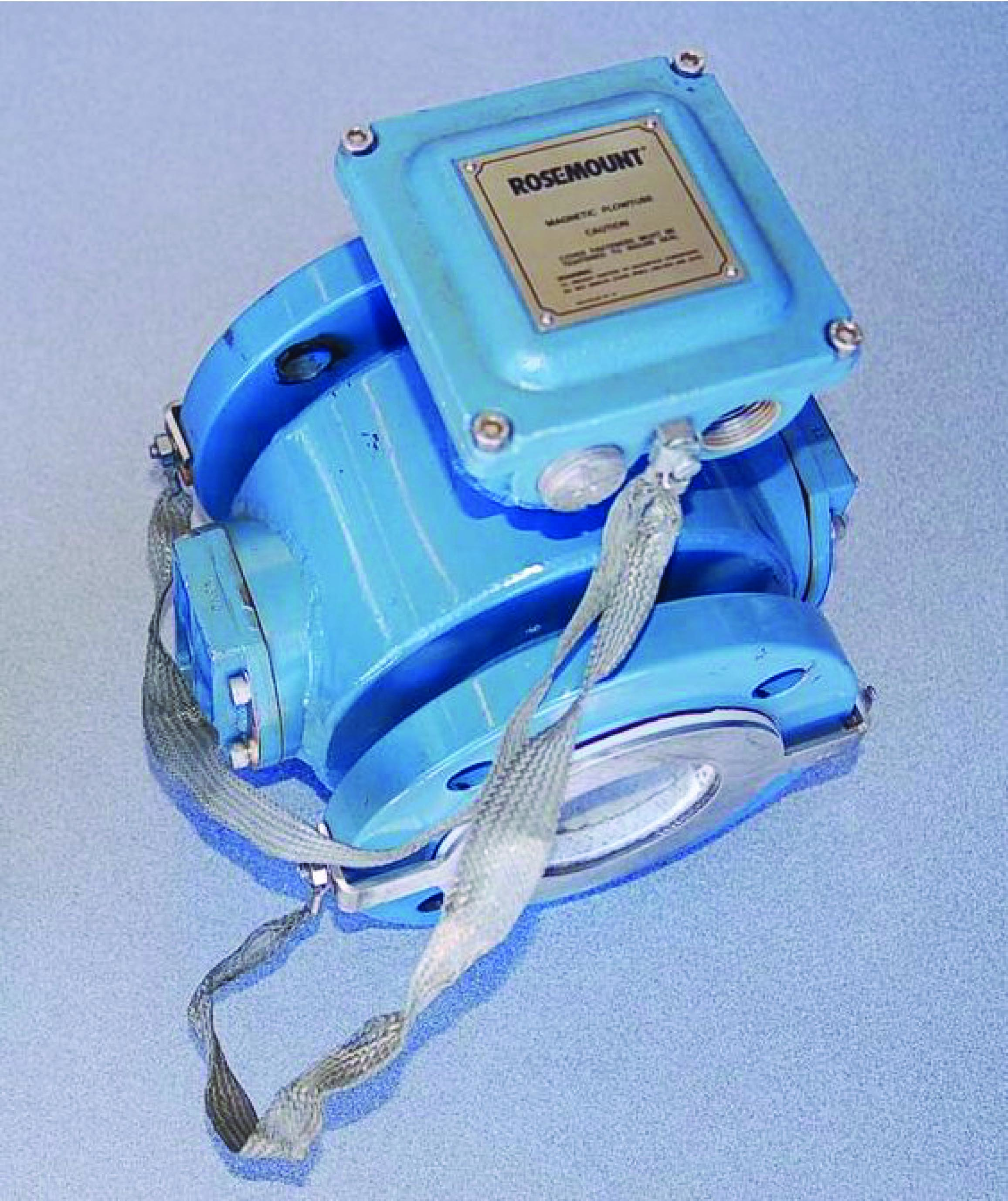
Note how both grounding straps attach to a common junction point on the flowtube housing. This common junction point should also be bonded to a functional earth ground when the flowtube is installed in the process line. On this particular flowtube you can see a stainless steel grounding ring on the face of the near flange, connected to one of the braided grounding straps. An identical grounding ring lays on the other flange, but it is not clearly visible in this photograph. These rings provide points of electrical contact with the liquid in installations where the pipe is made of plastic, or where the pipe is metal but lined with a plastic material for corrosion resistance.
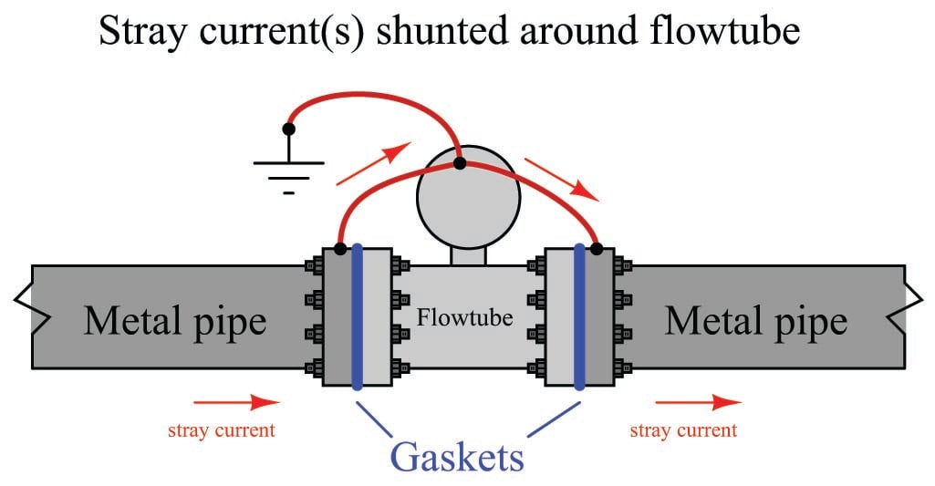
If the pipe connecting to a magnetic flowmeter’s flowtube is conductive (e.g. metal), grounding may be accomplished by joining the metal pipes’ flanges together with grounding straps to a common grounding point on the flowtube body as such:
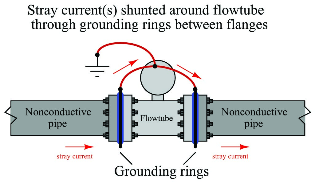
If the pipe connecting to a magnetic flowmeter’s flowtube is non-conductive (e.g. plastic) or conductive with an insulating lining (e.g. metal pipe with plastic lining), grounding to the pipe flanges will be pointless. In order for flowtube grounding to be effective, the grounding conductors must have electrical continuity to the fluid itself. Special grounding rings may be sandwiched between the flanges of non-conducting pipes to provide points of electrical contact with the fluid. These grounding rings are then joined together with grounding straps to a common grounding point on the flowtube body as such:
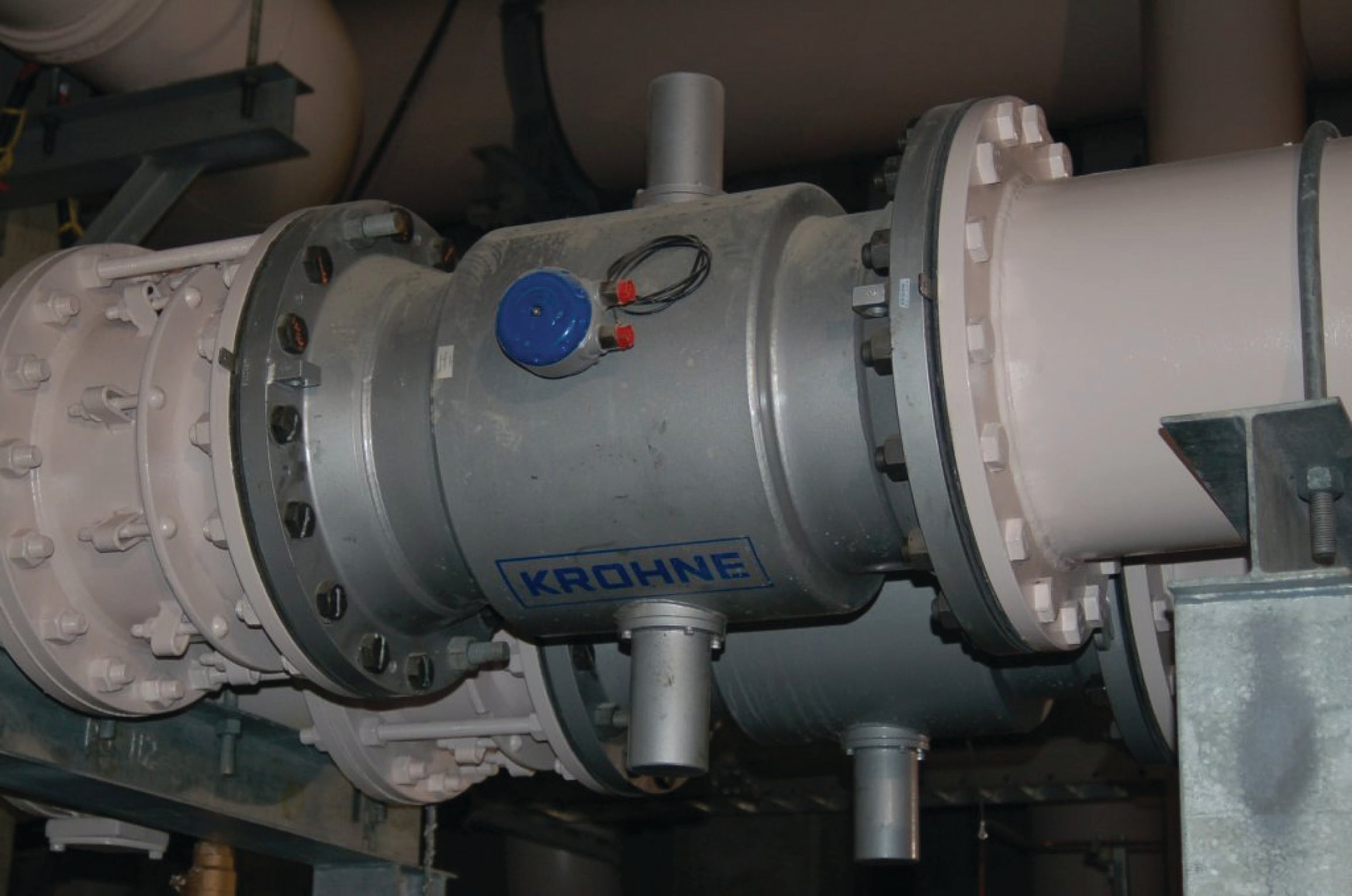
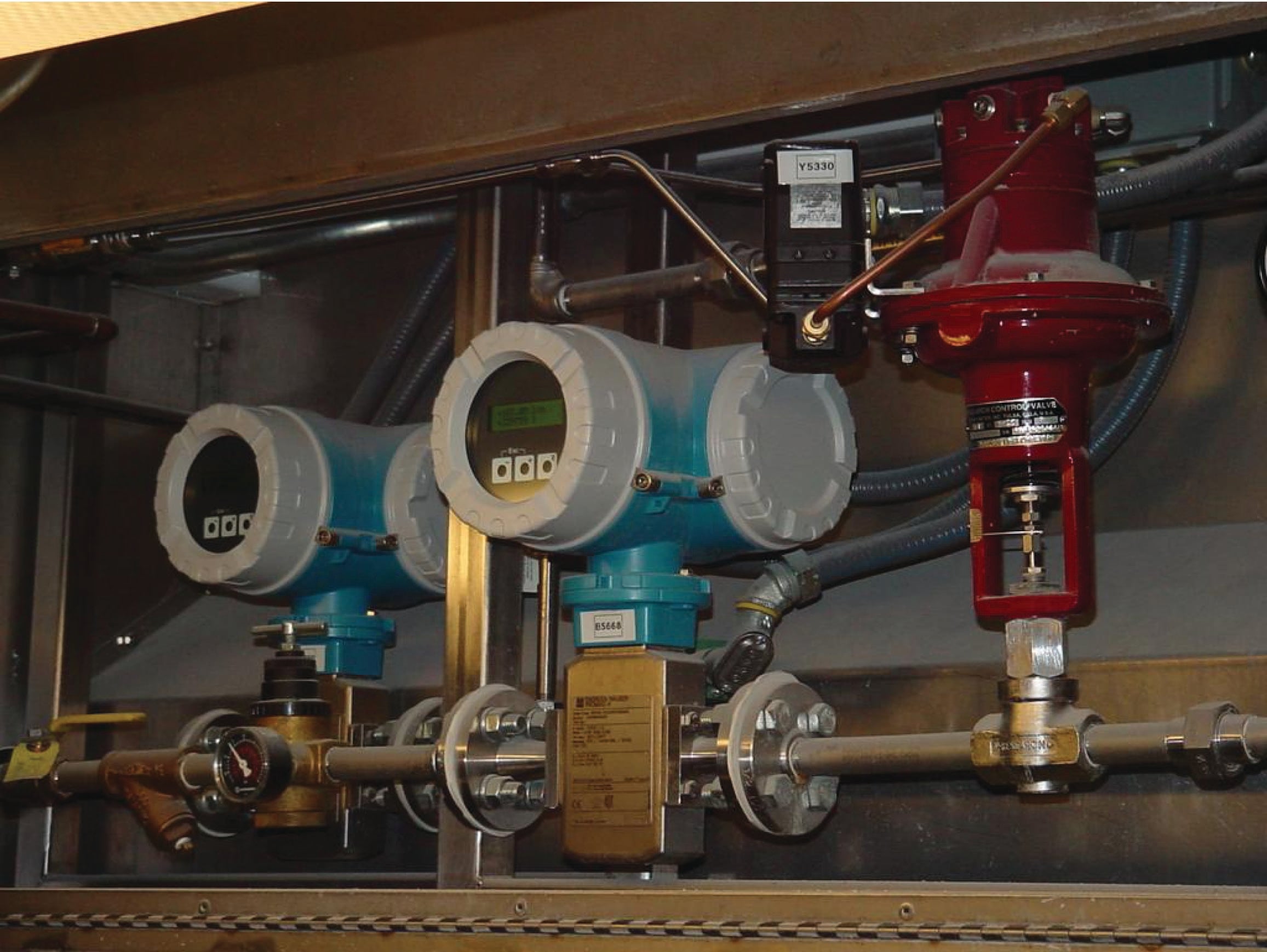
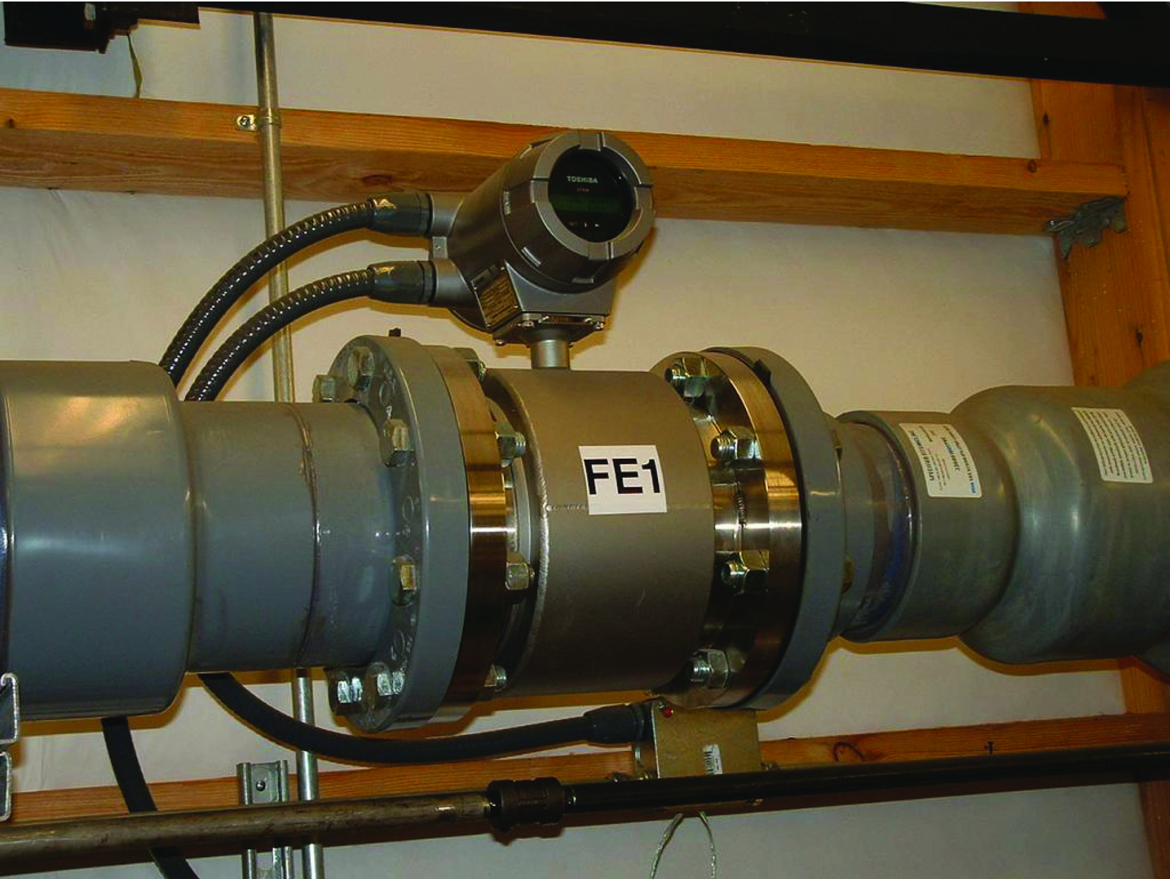
Some magnetic flowmeters have their signal conditioning electronics located integral to the flowtube assembly. A couple of examples are shown here (a pair of small Endress+Hauser flowmeters on the left and a large Toshiba flowmeter on the right):
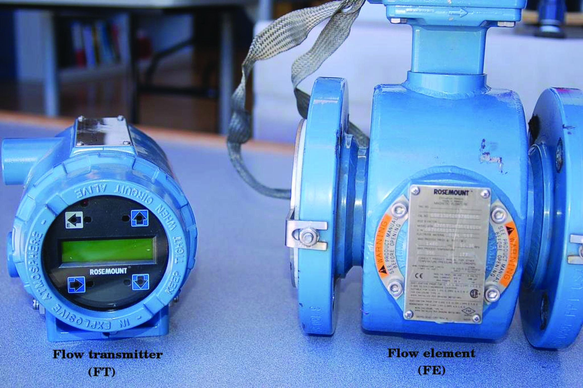
Other magnetic flowmeters have separate electronics and flowtube assemblies, connected together by shielded cable. In these installations, the electronics assembly is referred to as the flow transmitter (FT) and the flowtube as the flow element (FE):
This next photograph shows an enormous (36 inch diameter!) magnetic flow element (black) and flow transmitter (blue, behind the person’s hand shown for scale) used to measure wastewater flow at a municipal sewage treatment plant:
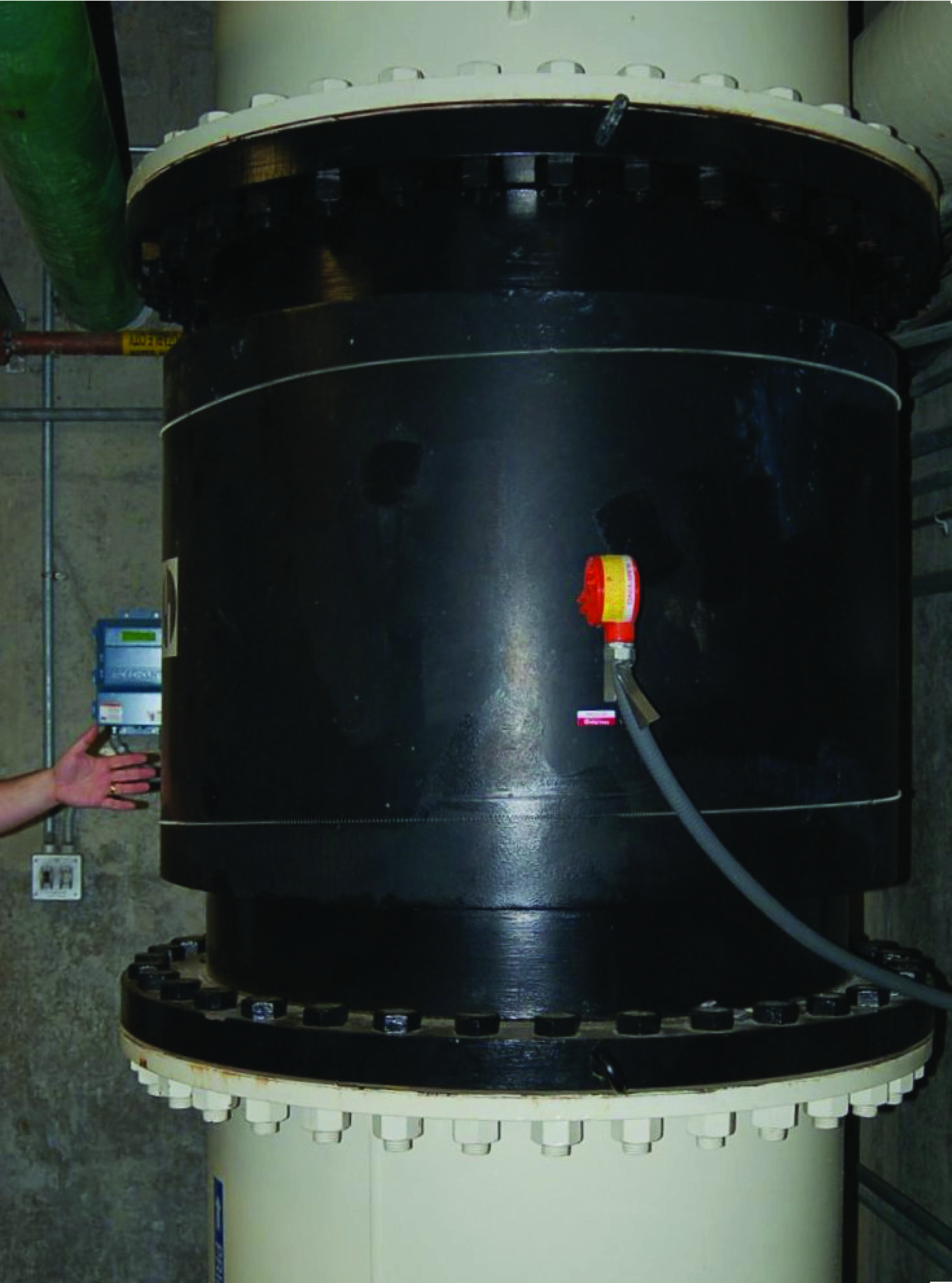
Note the vertical pipe orientation, ensuring constant contact between the electrodes and the water during flowing conditions.
While in theory a permanent magnet should be able to provide the necessary magnetic flux for a magnetic flowmeter to function, this is never done in industrial practice. The reason for this has to do with a phenomenon called polarization which occurs when a DC voltage is impressed across a liquid containing ions (electrically charged molecules). Electrically-charged molecules (ions) tend to collect near poles of opposite charge, which in this case would be the flowmeter electrodes. This “polarization” would soon interfere with detection of the motional EMF if a magnetic flowmeter were to use a constant magnetic flux such as that produced by a permanent magnet. A simple solution to this problem is to alternate the polarity of the magnetic field, so the motional EMF polarity also alternates and never gives the fluid ions enough time to polarize.
This is why magnetic flowmeter tubes always employ electromagnet coils to generate the magnetic flux instead of permanent magnets. The electronics package of the flowmeter energizes these coils with currents of alternating polarity, so as to alternate the polarity of the induced voltage across the moving fluid. Permanent magnets, with their unchanging magnetic polarities, would only be able to create an induced voltage with constant polarity, leading to ionic polarization and subsequent flow measurement errors.
A photograph of a Foxboro magnetic flowtube with one of the protective covers removed shows these wire coils clearly (in blue):
Perhaps the simplest form of coil excitation is when the coil is energized by 60 Hz AC power taken from the line power source, such as the case with this Foxboro flowtube. Since motional EMF is proportional to fluid velocity and to the flux density of the magnetic field, the induced voltage for such a coil will also be a 60 Hz sine wave whose amplitude varies with volumetric flow rate.
Unfortunately, if there is any stray electric current traveling through the liquid to produce erroneous voltage drops between the electrodes, chances are it will be 60 Hz AC as well. With the coil energized by 60 Hz AC, any such noise voltage may be falsely interpreted as fluid flow because the sensor electronics has no way to distinguish between 60 Hz noise in the fluid and a 60 Hz motional EMF caused by fluid flow.
A more sophisticated solution to this problem uses a pulsed excitation power source for the flowtube coils. This is called DC excitation by magnetic flowmeter manufacturers, which is a bit misleading because these “DC” excitation signals often reverse polarity, appearing more like an AC square wave on an oscilloscope display. The motional EMF for one of these flowmeters will exhibit the same waveshape, with amplitude once again being the indicator of volumetric flow rate. The sensor electronics can more easily reject any AC noise voltage because the frequency and waveshape of the noise (60 Hz, sinusoidal) will not match that of the flow-induced motional EMF signal.
The most significant disadvantage of pulsed-DC magnetic flowmeters is slower response time to changing flow rates. In an effort to achieve a “best-of-both-worlds” result, some magnetic flowmeter manufacturers produce dual-frequency flowmeters which energize their flowtube coils with two mixed frequencies: one below 60 Hz and one above 60 Hz. The resulting voltage signal intercepted by the electrodes is demodulated and interpreted as a flow rate.
Ultrasonic flowmeters
Ultrasonic flowmeters measure fluid velocity by passing high-frequency sound waves along the fluid flow path. Fluid motion influences the propagation of these sound waves, which may then be measured to infer fluid velocity. Two major sub-types of ultrasonic flowmeters exist: Doppler and transit-time. Both types of ultrasonic flowmeter work by transmitting a high-frequency sound wave into the fluid stream (the incident pulse) and analyzing the received pulse.
Doppler flowmeters exploit the Doppler effect, which is the shifting of frequency resulting from waves emitted by or reflected by a moving object. A common realization of the Doppler effect is the perceived shift in frequency of a horn’s report from a moving vehicle: as the vehicle approaches the listener, the pitch of the horn seems higher than normal; when the vehicle passes the listener and begins to move away, the horn’s pitch appears to suddenly “shift down” to a lower frequency. In reality, the horn’s frequency never changes, but the velocity of the approaching vehicle relative to the stationary listener acts to “compress” the sonic vibrations in the air. When the vehicle moves away, the sound waves are “stretched” from the perspective of the listener.
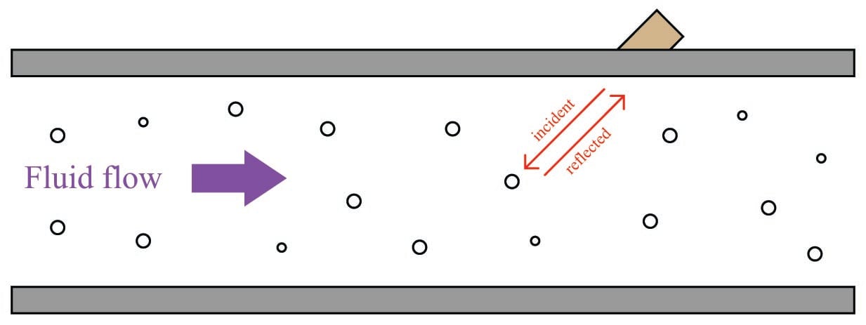
The same effect takes place if a sound wave is aimed at a moving object, and the echo’s frequency is compared to the transmitted (incident) frequency. If the reflected wave returns from a bubble advancing toward the ultrasonic transducer, the reflected frequency will be greater than the incident frequency. If the flow reverses direction and the reflected wave returns from a bubble traveling away from the transducer, the reflected frequency will be less than the incident frequency. This matches the phenomenon of a vehicle’s horn pitch seemingly increasing as the vehicle approaches a listener and seemingly decreasing as the vehicle moves away from a listener.
A Doppler flowmeter bounces sound waves off of bubbles or particulate material in the flow stream, measuring the frequency shift and inferring fluid velocity from the magnitude of that shift.
The requirement for there to be objects in the flow stream large enough to reflect sound waves limits Doppler ultrasonic flowmeters to liquid applications. “Dirty” liquids such as slurries and wastewater, or liquids carrying a substantial number of gas bubbles (e.g. carbonated beverages) are good candidate fluids for this technology. It is unrealistic to expect that any gas stream will be carrying liquid droplets or solid matter large enough to reflect strong echoes, and so Doppler flowmeters cannot be used to measure gas flow.
The mathematical relationship between fluid velocity (\(v\)) and the Doppler frequency shift (\(\Delta f\)) is as follows, for fluid velocities much less than the speed of sound through that fluid (\(v << c\)):
\[\Delta f = {{2vf \cos \theta} \over {c}}\]
Where,
\(\Delta f\) = Doppler frequency shift
\(v\) = Velocity of fluid (actually, of the particle reflecting the sound wave)
\(f\) = Frequency of incident sound wave
\(\theta\) = Angle between transducer and pipe centerlines
\(c\) = Speed of sound in the process fluid
Note how the Doppler effect yields a direct measurement of fluid velocity from each echo received by the transducer. This stands in marked contrast to measurements of distance based on time-of-flight (time domain reflectometry – where the amount of time between the incident pulse and the returned echo is proportional to distance between the transducer and the reflecting surface), such as in the application of ultrasonic liquid level measurement. In a Doppler flowmeter, the time delay between the incident and reflected pulses is irrelevant. Only the frequency shift between the incident and reflected signals matters. This frequency shift is also directly proportional to the velocity of flow, making the Doppler ultrasonic flowmeter a linear measurement device.
Re-arranging the Doppler frequency shift equation to solve for velocity (again, assuming \(v << c\)),
\[v = {{c \Delta f} \over {2 f \cos \theta}}\]
Knowing that volumetric flow rate is equal to the product of pipe area and the average velocity of the fluid (\(Q = A\overline{v}\)), we may re-write the equation to directly solve for calculated flow rate (\(Q\)):
\[Q = {{Ac \Delta f} \over {2 f \cos \theta}}\]
A very important consideration for Doppler ultrasonic flow measurement is that the calibration of the flowmeter varies with the speed of sound through the fluid (\(c\)). This is readily apparent by the presence of \(c\) in the above equation: as \(c\) increases, \(\Delta f\) must proportionately decrease for any fixed volumetric flow rate \(Q\). Since the flowmeter is designed to directly interpret flow rate in terms of \(\Delta f\), an increase in \(c\) causing a decrease in \(\Delta f\) will thus register as a decrease in \(Q\). This means the speed of sound for a fluid must be precisely known in order for a Doppler ultrasonic flowmeter to accurately measure flow.
The speed of sound through any fluid is a function of that medium’s density and bulk modulus (how easily it compresses):
\[c = \sqrt{B \over \rho}\]
Where,
\(c\) = speed of sound in a material (meters per second)
\(B\) = Bulk modulus (pascals, or newtons per square meter)
\(\rho\) = Mass density of fluid (kilograms per cubic meter)
Temperature affects liquid density, and composition (the chemical constituency of the liquid) affects bulk modulus. Thus, temperature and composition both are influencing factors for Doppler ultrasonic flowmeter calibration. Pressure is not a concern here, since pressure only affects the density of gases, and we already know Doppler flowmeters only function with liquids.
Following on the theme of requiring bubbles or particles of sufficient size, another limitation of Doppler ultrasonic flowmeters is their inability to measure flow rates of liquids that are too clean and too homogeneous. In such applications, the sound-wave reflections will be too weak to reliably measure. Such is also the case when the solid particles have a speed of sound too close to the that of the liquid, since reflection happens only when a sound wave encounters a material with a markedly different speed of sound. Doppler-type ultrasonic flowmeters are useless in applications where we cannot obtain strong sound-wave reflections.
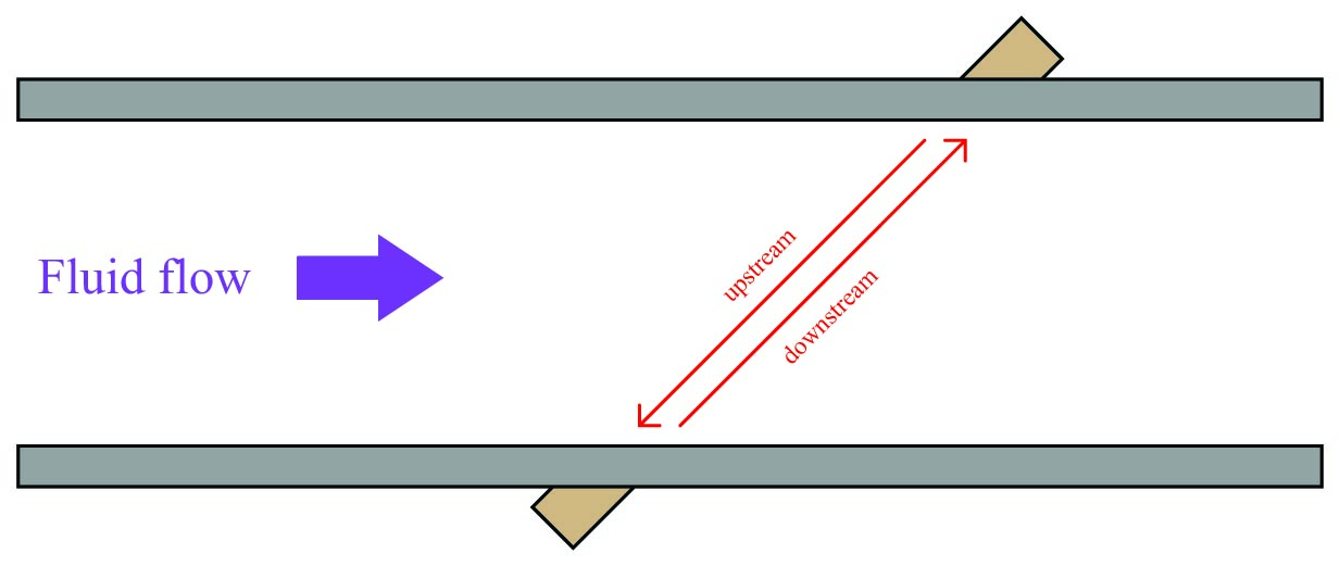
Transit-time flowmeters, sometimes called counterpropagation flowmeters, are an alternative to Doppler ultrasonic flowmeters. A transit-time ultrasonic flowmeter uses a pair of opposed sensors to measure the time difference between a sound pulse traveling with the fluid flow versus a sound pulse traveling against the fluid flow. Since the motion of fluid tends to carry a sound wave along, the sound pulse transmitted downstream will make the journey faster than a sound pulse transmitted upstream:
The rate of volumetric flow through a transit-time flowmeter is a simple function of the upstream and downstream propagation times:
\[Q = k {t_{up} - t_{down} \over (t_{up})(t_{down})}\]
Where,
\(Q\) = Calculated volumetric flow rate
\(k\) = Constant of proportionality
\(t_{up}\) = Time for sound pulse to travel from downstream location to upstream location (upstream, against the flow)
\(t_{down}\) = Time for sound pulse to travel from upstream location to downstream location (downstream, with the flow)
An interesting characteristic of transit-time velocity measurement is that the ratio of transit time difference over transit time product remains constant with changes in the speed of sound through the fluid. When this equation is cast into terms of path length (\(L\)), fluid velocity (\(v\)), and sound velocity (\(c\)), the equation simplifies to \(Q = {2kv \over L}\), proving that the transit-time flowmeter is linear just like the Doppler flowmeter, with the advantage of being immune to changes in the fluid’s speed of sound. Changes in bulk modulus resulting from changes in fluid composition, or changes in density resulting from compositional, temperature, or pressure variations therefore have little effect on a transit-time flowmeter’s accuracy.
Not only are transit-time ultrasonic flowmeters immune to changes in the speed of sound, but they are also able to measure that sonic velocity independent of the flow rate. The equation for calculating speed of sound based on upstream and downstream propagation times is as follows:
\[c = {L \over 2} \left({t_{up} + t_{down} \over (t_{up})(t_{down})}\right)\]
Where,
\(c\) = Calculated speed of sound in fluid
\(L\) = Path length
\(t_{up}\) = Time for sound pulse to travel from downstream location to upstream location (upstream, against the flow)
\(t_{down}\) = Time for sound pulse to travel from upstream location to downstream location (downstream, with the flow)
While not necessary or even particularly relevant for the direct purpose of flow measurement, this inference of the fluid’s speed of sound is nevertheless useful as a diagnostic tool. If the true speed of sound for the fluid is known either by direct laboratory measurement of a sample or by chemical analysis of a sample, this speed may be compared against the flowmeter’s reported speed of sound to check the flowmeter’s absolute transit time measurement accuracy. Certain problems within the sensors or within the sensor electronics may be detected in this way.
A requirement for reliable operation of a transit-time ultrasonic flowmeter is that the process fluid be free from gas bubbles or solid particles which might scatter or obstruct the sound waves. Note that this is precisely the opposite requirement of Doppler ultrasonic flowmeters, which require bubbles or particles to reflect sound waves. These opposing requirements neatly distinguish applications suitable for transit-time flowmeters from applications suitable for Doppler flowmeters, and also raise the possibility of using transit-time ultrasonic flowmeters on gas flowstreams as well as on liquid flowstreams.
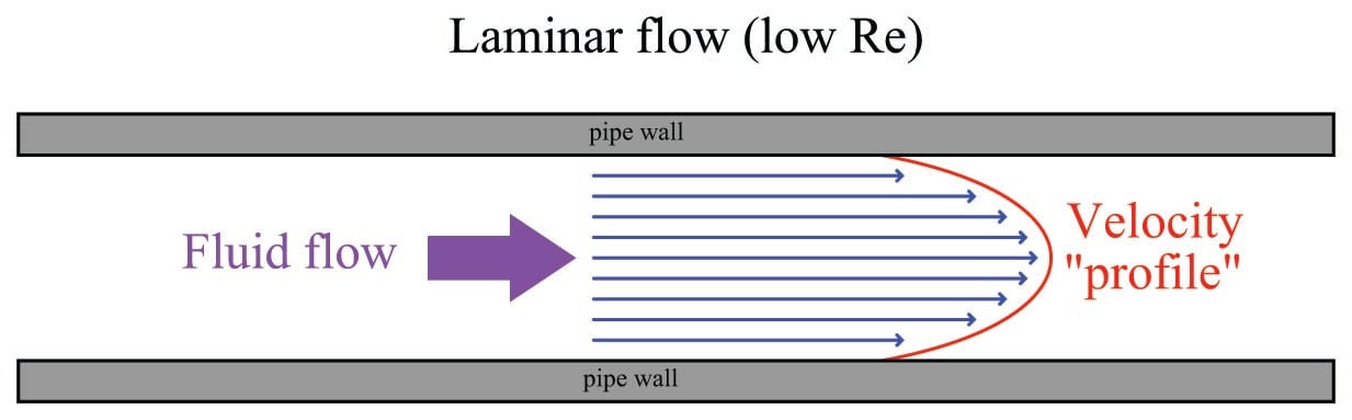
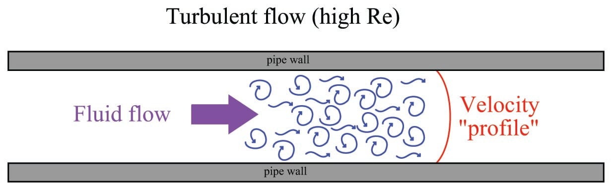
One potential problem with any ultrasonic flowmeter is being able to measure the true average fluid velocity when the flow profile changes with Reynolds number. If just one ultrasonic “beam” is used to probe the fluid velocity, the path this beam takes will likely see a different velocity profile as the flow rate changes (and the Reynolds number changes along with it). Recall the difference in fluid velocity profiles between low Reynolds number flows (left) and high Reynolds number flows (right):
A popular way to mitigate this problem is to use multiple sensor pairs, sending acoustic signals along multiple paths through the fluid (i.e. a multipath ultrasonic flowmeter), and to average the resulting velocity measurements. Dual-beam transit-time flowmeters have been in use for well over a decade at the time of this writing (2009), and one manufacturer even has a five beam ultrasonic flowmeter model which they claim maintains an accuracy of \(\pm\) 0.15% through the laminar-to-turbulent flow regime transition. A simplified illustration of a Daniel four-beam (or four “chord”) ultrasonic flowmeter is shown here:
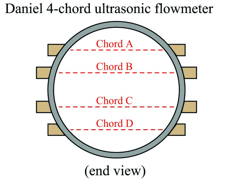
Multipath ultrasonic flowmeters, by virtue of measuring more than one sound wave path through the fluid, also have the ability to detect irregular flow profiles. Each sonic path between sensor pairs in a transit-time ultrasonic flowmeter, called a chord, measures flow velocity. The velocities reported for each chord may be compared to the flowmeter’s calculated average flow velocity, and expressed as velocity ratios. A particular chord measuring a velocity greater than the flowmeter’s average will report a velocity ratio greater than one (\(>1\)), whereas a chord measuring a velocity less than the meter’s average will report a velocity ratio less than one (\(<1\)). In the Daniel four-chord ultrasonic flowmeter, two chords (B and C) measure velocity near the center of the pipe while the others (A and D) measure velocity closer to the pipe walls. In normal operation, the center chord velocity ratios should exceed the outer chord velocity ratios by a small amount, since the flow profiles of laminar and turbulent flow regimes alike exhibit a greater velocity at the center of a pipe than near the walls of a pipe.
Another parameter called profile factor expresses the chord velocity factors as a ratio, inner velocity factors over outer velocity factors: \({B + C} \over {A + D}\), a number which should always exceed one (\(>1\)). The exact value of this profile factor varies with the flowmeter’s installation, and may shift over time if the flow profile shifts for some reason (e.g. partial blockage in a flow conditioner, piping change, accumulation of debris on pipe wall). For example, a pipe accumulating dirt or other solid material on its walls over time will tend to slow down the velocity of fluid near the walls compared to the velocity of fluid in the center. This has the effect of decreasing chord A and D velocity ratios while increasing chord B and C velocity ratios, which in turn increases the profile factor value. In this regard, the profile factor value for an operating flowmeter may be an important diagnostic tool, indicating some physical abnormality within the piping.
As previously mentioned, it is possible for a transit-time ultrasonic flowmeter to measure the speed of sound through the fluid from the sum of the upstream and downstream transit times. Multipath transit-time flowmeters may use this feature to cross-check calculated speed of sound values measured by each chord, as a self-diagnostic tool. Since each chord measures the same gas composition, each chord’s calculated speed of sound should be exactly equal. Significant differences in calculated speed of sound between chords suggests a failure in the acoustic sensor(s) or electronics for the errant chord.
Some modern ultrasonic flowmeters have the ability to switch back and forth between Doppler and transit-time (counterpropagation) modes, automatically adapting to the fluid being sensed. This capability enhances the suitability of ultrasonic flowmeters to a wider range of process applications.
Ultrasonic flowmeters are adversely affected by swirl and other large-scale fluid disturbances, and as such may require substantial lengths of straight pipe upstream and downstream of the measurement flowtube to stabilize the flow profile.
Like magnetic flowmeters, ultrasonic flowmeters are completely non-obstructive, which means they exhibit extremely low permanent pressure loss and will not accumulate debris.
Advances in ultrasonic flow measurement technology have reached a point where it is now feasible to consider ultrasonic flowmeters for custody transfer measurement of natural gas. The American Gas Association has released a report specifying the use of multipath transit-time ultrasonic flowmeters in this capacity (Report #9). As with the AGA’s #3 (orifice plate) and #7 (turbine) high-accuracy gas flow measurement standards, the AGA9 standard requires the addition of pressure and temperature instruments on the gas line to measure gas pressure and temperature in order to calculate flow either in units of mass or in units of standardized volume (e.g. SCFM). The measurement of temperature and pressure for a transit-time ultrasonic flowmeter has nothing to do with correcting errors within the meter itself, since we know transit-time flowmeters are inherently immune to changes in gas density or composition. Temperature and pressure measurements are necessary for custody transfer applications simply because ultrasonic flowmeters, like turbine flowmeters, measure only volumetric flow. The fair sale and purchase of a gas requires measurement of molecular quantity, not just volume, which is why a flow computer requires measurements of pressure and temperature in order to convert the ultrasonic flowmeter’s volumetric output to either mass flow or standardized volumetric flow.
A unique advantage of ultrasonic flow measurement is the ability to measure flow through the use of temporary clamp-on sensors rather than a specialized flowtube with built-in ultrasonic transducers. While clamp-on sensors are not without their share of problems, they constitute an excellent solution for certain flow measurement applications.
An important criterion for successful application of a clamp-on flowmeter is that the pipe material be homogeneous in nature, to efficiently conduct sound waves between the process fluid and the clamp-on transducers. Porous pipe materials such as clay and concrete are therefore unsuitable for clamp-on ultrasonic flow measurement.
Optical flowmeters
A relatively recent development in industrial flow measurement is the use of light to measure the velocity of a fluid through a pipe. One such technology referred to as Laser-Two-Focus (L2F) uses two laser beams to detect the passage of any light-scattering particles carried along by the moving fluid:
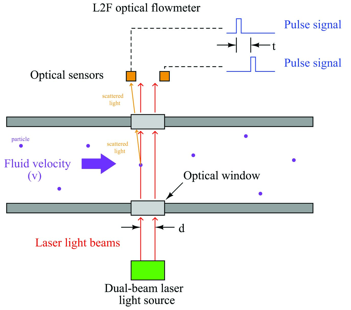
\[v = {d \over t}\]
Where,
\(v\) = Velocity of particle
\(d\) = Distance separating laser beams
\(t\) = Time difference between sensor pulses
As a particle passes through each laser beam, it redirects the light away from its normal straight-line path in such a way that an optical sensor (one per beam) detects up the scattered light and generates a pulse signal. As that same particle passes through the second beam, the scattered light excites a second optical sensor to generate a corresponding pulse signal. The time delay between two successive pulses is inversely proportional to the velocity of that particle. This technique is analogous to the that used by law-enforcement officers to measure the speed of a vehicle on a highway when viewed from an aircraft: measure how much time elapses as the vehicle passes between two marks on the road spaced a known distance from each other.
L2F flowmeters of course rely on the continual presence of light-scattering particles within the fluid. These particles could be either liquid droplets or solids within a gas stream, or they could be solid particles or bubbles in a liquid stream.
An alternative to passing laser beams across the entire width of the pipe is to shrink the assembly down to the size of a probe which may be inserted into a pipe. While minimizing installation and maintenance costs, this approach suffers the disadvantage of sensing velocity at only one point within the flow stream, much like a classic Pitot tube. In order to obtain a measurement of bulk (average) fluid velocity, the raw velocity measurement provided by the sensor must be corrected based on the expected Reynolds number for the process fluid, which is why insertion L2F flowmeters are equipped with pressure and temperature transmitters in addition to the optical probe. When the three measurements (pressure, temperature, and velocity at the probe) are combined, the Reynolds number may be calculated which then predicts how “flat” (consistent) the velocity profile is for the fluid stream:
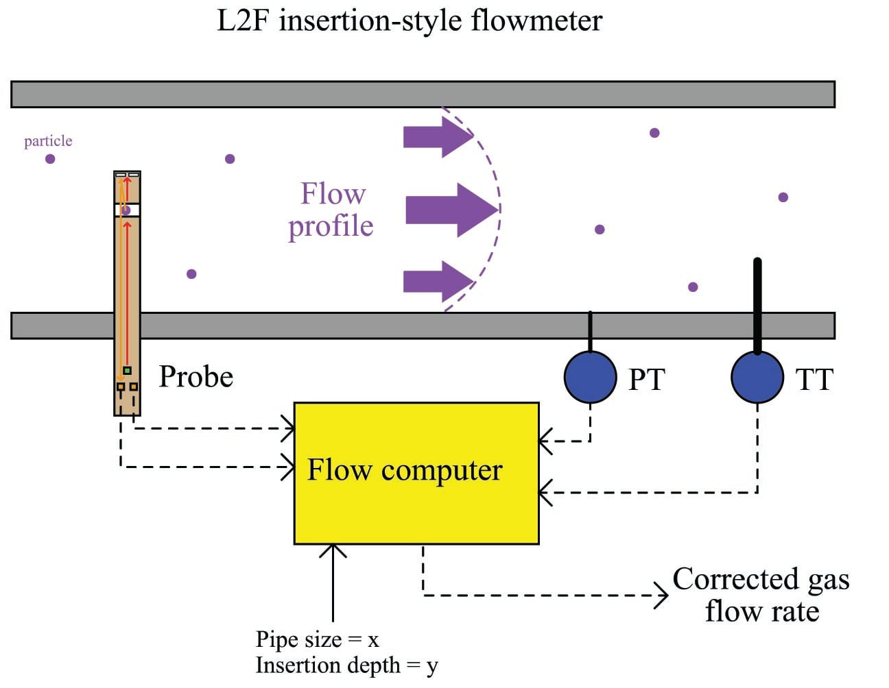
For example, if the probe velocity, pressure, temperature, and dimensional parameters indicate a high Reynolds number, it means the velocity profile will be relatively flat, and thus the single-point velocity measurement at the probe will be a fair representation of velocity across the entire width of the pipe. However, if the parameters indicate a low Reynolds number, it means the velocity profile will have a more pronounced “bullet” shape, and therefore the velocities near the pipe walls will be substantially less than the velocity at the center. The flow computer uses this predicted velocity profile to interpret the probe’s single-point velocity measurement and calculate the average velocity of the entire flowstream.
A more sophisticated technique for optical flow measurement relies on the principle of scintillation, whereby the fluid itself warps the path of light passing through, rather than entrained particulate matter scattering the light. Scintillation is the same phenomenon responsible for the “twinkling” of stars and city lights viewed from a long distance: as air passes between the light and the observer, pockets of air having different density (due to differences in temperature) and/or sufficient turbulence cause some of the light to be refracted away from an otherwise straight-line path, making it appear as though the light source is randomly vibrating or oscillating. In fact, the phenomenon of scintillation has been used for the measurement of air velocity (anemometry) for many years before its application to industrial flow measurement.
Velocity measurements are inferred by a scintillation flowmeter much the same as they are by an L2F optical flowmeter: measuring the time difference between two sensors’ detection of the same scintillation pattern. Therefore, the scintillation flowmeter applies the same basic formula \(v = {d \over t}\) to calculate fluid velocity. A simplified diagram of a scintillation flowmeter is shown here:
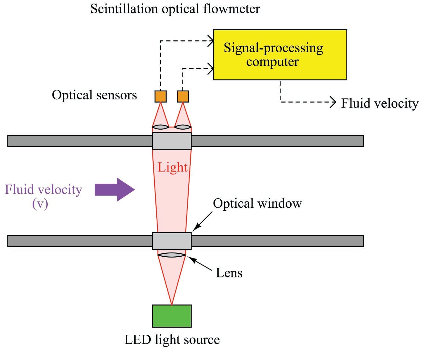
Scintillation-style optical flowmeters require a long optical path in order to maximize the angle at which light will be refracted. Thus, they function best when used to measure across the full diameter of a pipe. An interesting feature of this flowmeter technology is that it functions best when the flow regime is highly turbulent, since increased fluid turbulence leads to greater scintillation.
Both L2F and scintillation flowmeters have phenomenal turndown ratios. At the low end of the velocity measurement range, an L2F meter is limited by the number of particles entrained in the flow stream and also by the random motions of particles which might be misinterpreted by the flowmeter as bulk motion of the fluid. Scintillation flowmeters are limited at the low end of their measurement range by loss of turbulence, which of course is one of the driving mechanisms of the scintillation effect. However, it should be noted that in both cases the low-velocity measuring limit is quite low in comparison to other types of flowmeters. With no moving parts and using light as the sensing medium, the upper limit for an optical flowmeter can extend into supersonic velocities. This combination of excellent low-velocity and high-velocity sensing yields practical turndown ratios of 1000:1 or more.
Optical flowmeters have been successfully used in one of the more challenging industrial flow measurement applications in existence: flare gas flow metering. A “flare” is a continually-ignited burner used as a safety relief point for flammable gases in industries such as petroleum production and refining where a need exists to occasionally vent these gases to the atmosphere:
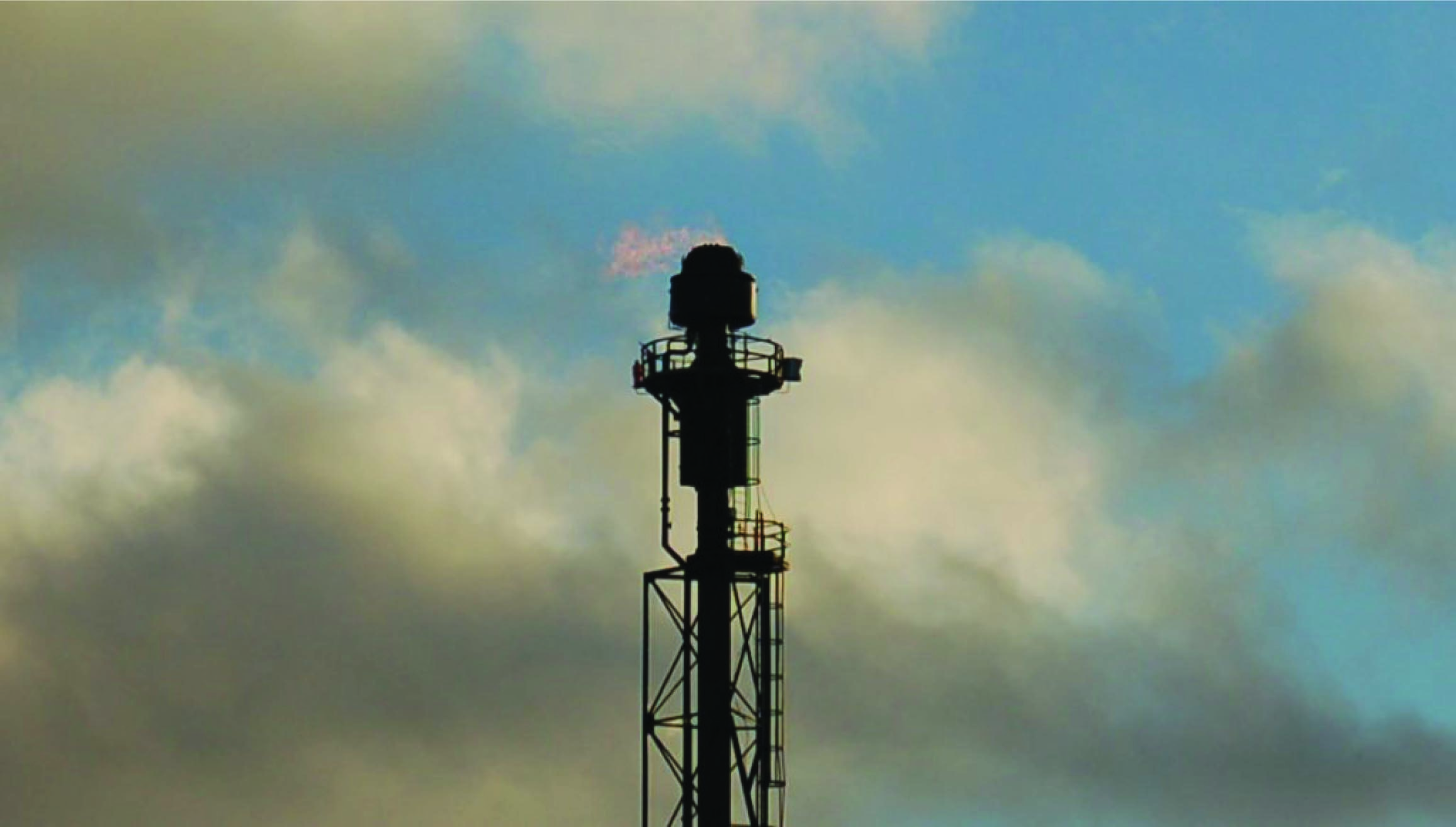
Ideally, flares operate with no flow of gas to them except during emergency conditions, and then when there is an emergency the flow rate can be very high. In order to accurately measure the low “quiescent” flow of gas to a flare during non-emergency operation (due to pressure relief valve leakage and other inefficiencies) while still being able to register full flow rates during emergencies, the flowmeter must have an extremely large turndown ratio (rangeability).
Gas sent to a flare typically varies widely in composition, temperature, and pressure, especially when multiple processing units share a common flare. The random variability of the gas eliminates many types of flowmeters from consideration. Pressure-based flowmeters such as orifice plates suffer from calibration errors due to density changes, as well as poor turndown ratio. Thermal mass flowmeters suffer from calibration errors due to changes in the specific heat value of the flare gas. Velocity-based gas flowmeters (e.g. turbine, vortex, ultrasonic) are not affected by compositional changes to the extent that pressure-based and thermal flowmeters are, but few exhibit the degree of turndown necessary to accurately measure the full range of flare gas flow. Multi-path transit-time ultrasonic flowmeters show promise in this challenging application, but their relatively high cost (especially at the large pipe diameters typical of flare headers) is a limiting factor.
