 Facebook
 Google
 GitHub
 Linkedin
Pressure-based Flowmeters
All masses require force to accelerate (we can also think of this in terms of the mass generating a reaction force as a result of being accelerated). This is quantitatively expressed by Newton’s Second Law of Motion:
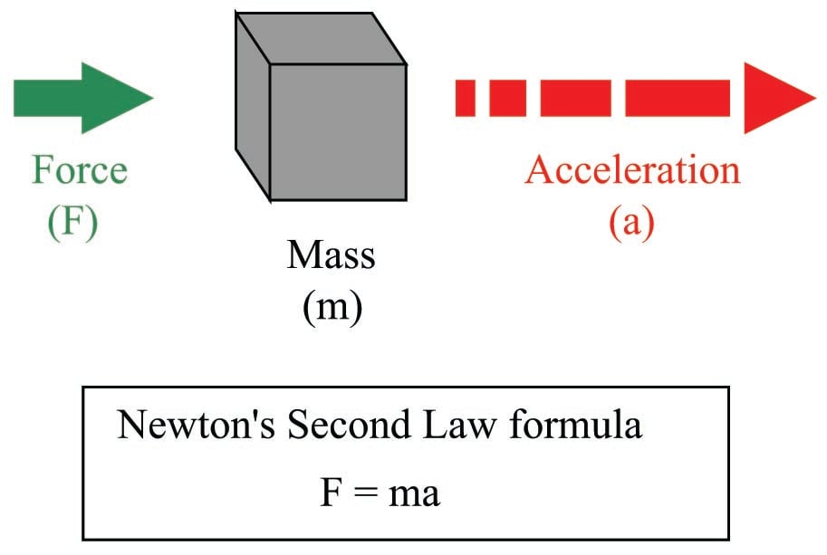
All fluids possess mass, and therefore require force to accelerate just like solid masses. If we consider a quantity of fluid confined inside a pipe, with that fluid quantity having a mass equal to its volume multiplied by its mass density (\(m = \rho V\), where \(\rho\) is the fluid’s mass per unit volume), the force required to accelerate that fluid “plug” would be calculated just the same as for a solid mass:
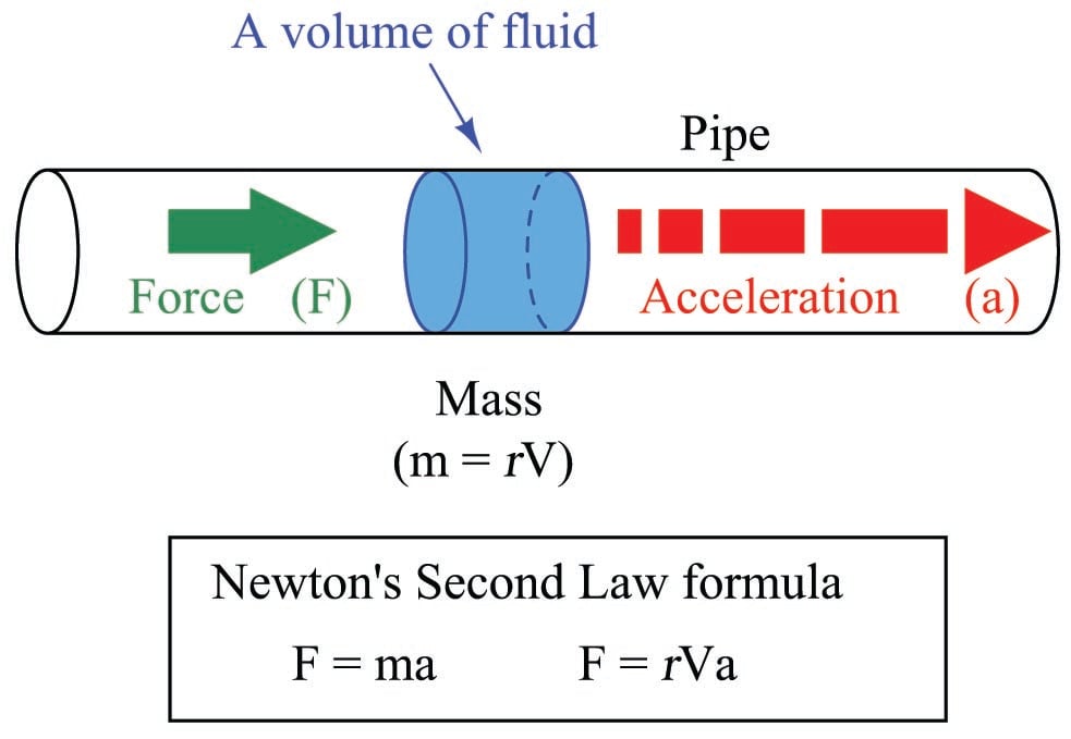
Since this accelerating force is applied on the cross-sectional area of the fluid plug, we may express it as a pressure, the definition of pressure being force per unit area:
\[F = \rho V a\]
\[{F \over A} = \rho {V \over A} a\]
\[P = \rho {V \over A} a\]
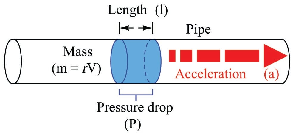
Since the rules of algebra required we divide both sides of the force equation by area, it left us with a fraction of volume over area (\(V \over A\)) on the right-hand side of the equation. This fraction has a physical meaning, since we know the volume of a cylinder divided by the area of its circular face is simply the length of that cylinder:
\[P = \rho {V \over A} a\]
\[P = \rho l a\]
When we apply this to the illustration of the fluid mass, it makes sense: the pressure described by the equation is actually a differential pressure drop from one side of the fluid mass to the other, with the length variable (\(l\)) describing the spacing between the differential pressure ports:
This tells us we can accelerate a “plug” of fluid by applying a difference of pressure across its length. The amount of pressure we apply will be in direct proportion to the density of the fluid and its rate of acceleration. Conversely, we may measure a fluid’s rate of acceleration by measuring the pressure developed across a distance over which it accelerates.
We may easily force a fluid to accelerate by altering its natural flow path. The difference of pressure generated by this acceleration will indirectly indicate the rate of acceleration. Since the acceleration we see from a change in flow path is a direct function of how fast the fluid was originally moving, the acceleration (and therefore the pressure drop) indirectly indicates fluid flow rate.
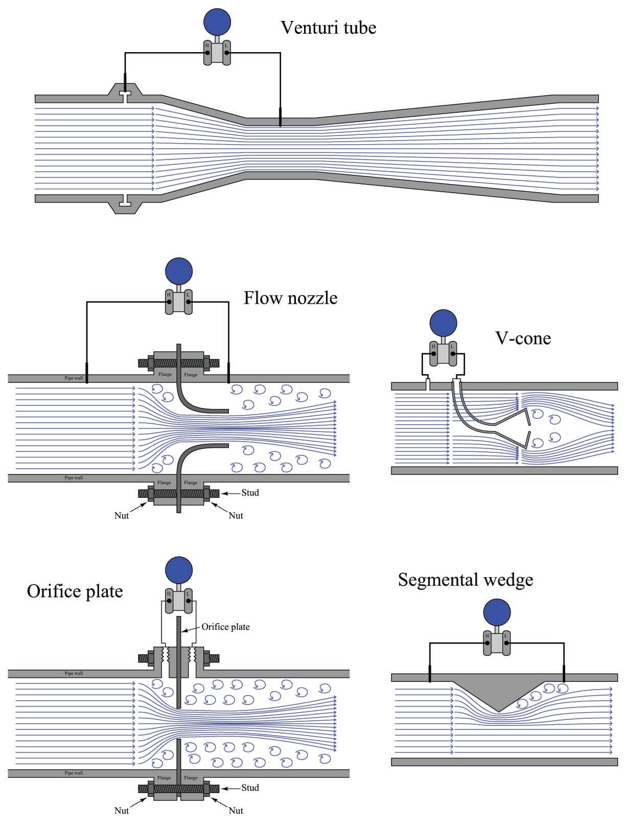
A very common way to cause linear acceleration in a moving fluid is to pass the fluid through a constriction in the pipe, thereby increasing its velocity (remember that the definition of acceleration is a change in velocity). The following illustrations show several devices used to linearly accelerate moving fluids when placed in pipes, with differential pressure transmitters connected to measure the pressure drop resulting from this acceleration:
Another way we may accelerate a fluid is to force it to turn a corner through a pipe fitting called an elbow. This will generate radial acceleration, causing a pressure difference between the outside and inside of the elbow which may be measured by a differential pressure transmitter:
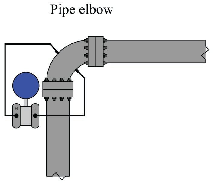
The pressure tap located on the outside of the elbow’s turn registers a greater pressure than the tap located on the inside of the elbow’s turn, due to the inertial force of the fluid’s mass being “flung” to the outside of the turn as it rounds the corner.
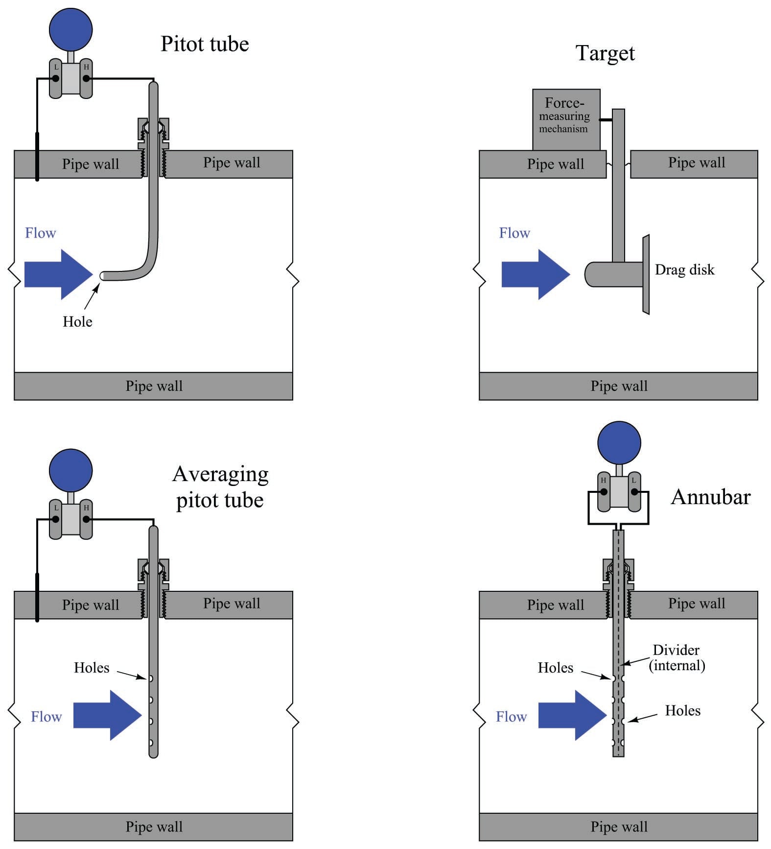
Yet another way to cause a change in fluid velocity is to force it to decelerate by bringing a portion of it to a full stop. The pressure generated by this deceleration (called the stagnation pressure) tells us how fast it was originally flowing. A few devices working on this principle are shown here:
The following subsections in this flow measurement chapter explore different primary sensing elements (PSE’s) used to generate differential pressure in a moving fluid stream. Despite their very different designs, they all operate on the same fundamental principle: causing a fluid to accelerate or decelerate by forcing a change in its flow path, and thus generating a measurable pressure difference. The following subsection will introduce a device called a venturi tube used to measure fluid flow rates, and derive mathematical relationships between fluid pressure and flow rate starting from basic physical conservation laws.
Venturi tubes and basic principles
The standard “textbook example” flow element used to create a pressure change by accelerating a fluid stream is the venturi tube: a pipe purposefully narrowed to create a region of low pressure. As shown previously, venturi tubes are not the only structure capable of producing a flow-dependent pressure drop. You should keep this in mind as we proceed to derive equations relating flow rate with pressure change: although the venturi tube is the canonical form, the exact same mathematical relationship applies to all flow elements generating a pressure drop by accelerating fluid, including orifice plates, flow nozzles, V-cones, segmental wedges, pipe elbows, pitot tubes, etc.
If the fluid going through the venturi tube is a liquid under relatively low pressure, we may vividly show the pressure at different points in the tube by means of piezometers, which are transparent tubes allowing us to view liquid column heights. The greater the height of liquid column in the piezometer, the greater the pressure at that point in the flowstream:
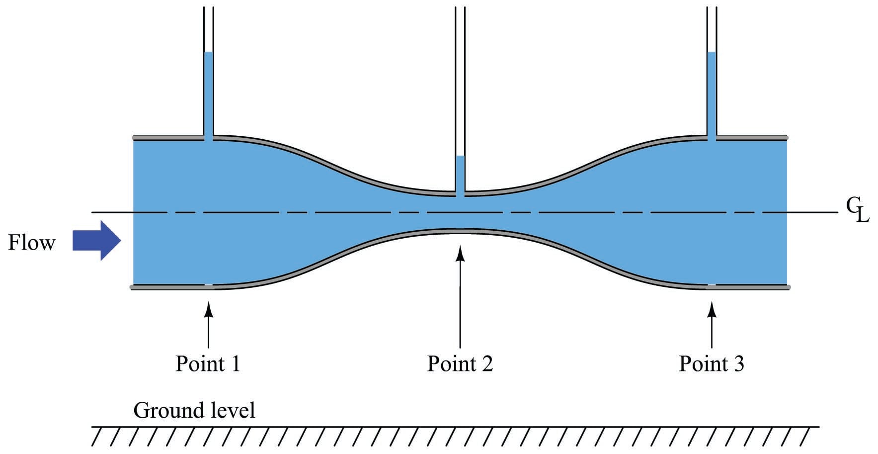
As indicated by the piezometer liquid heights, pressure at the constriction (point 2) is the least, while pressures at the wide portions of the venturi tube (points 1 and 3) are the greatest. This is a counter-intuitive result, but it has a firm grounding in the physics of mass and energy conservation. If we assume no energy is added (by a pump) or lost (due to friction) as fluid travels through this pipe, then the Law of Energy Conservation describes a situation where the fluid’s energy must remain constant at all points in the pipe as it travels through. If we assume no fluid joins this flowstream from another pipe, or is lost from this pipe through any leaks, then the Law of Mass Conservation describes a situation where the fluid’s mass flow rate must remain constant at all points in the pipe as it travels through.
So long as fluid density remains fairly constant, fluid velocity must increase as the cross-sectional area of the pipe decreases, as described by the Law of Continuity (see section [Law of Continuity] beginning on page for more details on this concept):
\[A_1 \overline{v_1} = A_2 \overline{v_2}\]
Rearranging variables in this equation to place velocities in terms of areas, we get the following result:
\[{\> \overline{v_2} \> \over \> \overline{v_1} \>} = {A_1 \over A_2}\]
This equation tells us that the ratio of fluid velocity between the narrow throat (point 2) and the wide mouth (point 1) of the pipe is the same ratio as the mouth’s area to the throat’s area. So, if the mouth of the pipe had an area 5 times as great as the area of the throat, then we would expect the fluid velocity in the throat to be 5 times as great as the velocity at the mouth. Simply put, the narrow throat causes the fluid to accelerate from a lower velocity to a higher velocity.
We know from our study of energy in physics that kinetic energy is proportional to the square of a mass’s velocity (\(E_k = {1 \over 2}mv^2\)). If we know the fluid molecules increase velocity as they travel through the venturi tube’s throat, we may safely conclude that those molecules’ kinetic energies must increase as well. However, we also know that the total energy at any point in the fluid stream must remain constant, because no energy is added to or taken away from the stream in this simple fluid system. Therefore, if kinetic energy increases at the throat, potential energy must correspondingly decrease to keep the total amount of energy constant at any point in the fluid.
Potential energy may be manifest as height above ground, and/or as pressure in a fluid system. Since this venturi tube is level with the ground, there cannot be a height change to account for a change in potential energy. Therefore, there must be a change of pressure (\(P\)) as the fluid travels through the venturi throat. The Laws of Mass and Energy Conservation invariably lead us to this conclusion: fluid pressure must decrease as it travels through the narrow throat of the venturi tube.
Conservation of energy at different points in a fluid stream is neatly expressed in Bernoulli’s Equation as a constant sum of elevation, pressure, and velocity “heads” (see section 2.11.13 beginning on page for more details on this concept):
\[z_1 \rho g + {v_1^2 \rho \over 2} + P_1 = z_2 \rho g + {v_2^2 \rho \over 2} + P_2\]
Where,
\(z\) = Height of fluid (from a common reference point, usually ground level)
\(\rho\) = Mass density of fluid
\(g\) = Acceleration of gravity
\(v\) = Velocity of fluid
\(P\) = Pressure of fluid
We will use Bernoulli’s equation to develop a precise mathematical relationship between pressure and flow rate in a venturi tube. To simplify our task, we will hold to the following assumptions for our venturi tube system:
- No energy lost or gained in the venturi tube (all energy is conserved)
- No mass lost or gained in the venturi tube (all mass is conserved)
- Fluid is incompressible
- Venturi tube centerline is level (no height changes to consider)
Applying the last two assumptions to Bernoulli’s equation, we see that the “elevation head” term drops out of both sides, since \(z\), \(\rho\), and \(g\) are equal at all points in the system:
\[{v_1^2 \rho \over 2} + P_1 = {v_2^2 \rho \over 2} + P_2\]
Now we will algebraically re-arrange this equation to show pressures at points 1 and 2 in terms of velocities at points 1 and 2:
\[{v_2^2 \rho \over 2} - {v_1^2 \rho \over 2} = P_1 - P_2\]
Factoring \(\rho \over 2\) out of the velocity head terms:
\[{\rho \over 2} (v_2^2 - v_1^2) = P_1 - P_2\]
The Continuity equation shows us the relationship between velocities \(v_1\) and \(v_2\) and the areas at those points in the venturi tube, assuming constant density (\(\rho\)):
\[A_1 v_1 = A_2 v_2\]
Specifically, we need to re-arrange this equation to define \(v_1\) in terms of \(v_2\) so we may substitute into Bernoulli’s equation:
\[v_1 = \left({A_2 \over A_1}\right) v_2\]
Performing the algebraic substitution:
\[{\rho \over 2} (v_2^2 - \left[\left({A_2 \over A_1}\right) v_2\right]^2) = P_1 - P_2\]
Distributing the “square” power:
\[{\rho \over 2} (v_2^2 - \left({A_2 \over A_1}\right)^2 v_2^2) = P_1 - P_2\]
Factoring \(v_2^2\) out of the outer parentheses set:
\[{\rho v_2^2 \over 2} (1 - \left({A_2 \over A_1}\right)^2) = P_1 - P_2\]
Solving for \(v_2\), step by step:
\[{\rho v_2^2 \over 2} = \left({1 \over {1 - \left({A_2 \over A_1}\right)^2}}\right) (P_1 - P_2)\]
\[\rho v_2^2 = 2 \left({1 \over {1 - \left({A_2 \over A_1}\right)^2}}\right) (P_1 - P_2)\]
\[v_2^2 = 2 \left({1 \over {1 - \left({A_2 \over A_1}\right)^2}}\right) \left({{P_1 - P_2} \over \rho}\right)\]
\[v_2 = \sqrt{2} {1 \over \sqrt{1 - \left({A_2 \over A_1}\right)^2}} \sqrt{{P_1 - P_2} \over \rho}\]
The result shows us how to solve for fluid velocity at the venturi throat (\(v_2\)) based on a difference of pressure measured between the mouth and the throat (\(P_1 - P_2\)). We are only one step away from a volumetric flow equation here, and that is to convert velocity (\(v\)) into flow rate (\(Q\)). Velocity is expressed in units of length per time (feet or meters per second or minute), while volumetric flow is expressed in units of volume per time (cubic feet or cubic meters per second or minute). Simply multiplying throat velocity (\(v_2\)) by throat area (\(A_2\)) will give us the result we seek:
General flow/area/velocity relationship:
\[Q = Av\]
Equation for throat velocity:
\[v_2 = \sqrt{2} {1 \over \sqrt{1 - \left({A_2 \over A_1}\right)^2}} \sqrt{{P_1 - P_2} \over \rho}\]
Multiplying both sides of the equation by throat area:
\[A_2 v_2 = \sqrt{2} A_2 {1 \over \sqrt{1 - \left({A_2 \over A_1}\right)^2}} \sqrt{{P_1 - P_2} \over \rho}\]
Now we have an equation solving for volumetric flow (\(Q\)) in terms of pressures and areas:
\[Q = \sqrt{2} A_2 {1 \over \sqrt{1 - \left({A_2 \over A_1}\right)^2}} \sqrt{{P_1 - P_2} \over \rho}\]
[Ideal flow equation]
Please note how many constants we have in this equation. For any given venturi tube, the mouth and throat areas (\(A_1\) and \(A_2\)) will be fixed. This means nearly half the variables found within this rather long equation are actually constant for any given venturi tube, and therefore do not change with pressure, density, or flow rate. Knowing this, we may re-write the equation as a simple proportionality:
\[Q \propto \sqrt{{P_1 - P_2} \over \rho}\]
To make this a more precise mathematical statement, we may insert a constant of proportionality (\(k\)) and once more have a true equation to work with:
\[Q = k \sqrt{{P_1 - P_2} \over \rho}\]
Volumetric flow calculations
As we saw in the previous subsection, we may derive a relatively simple equation for predicting flow through a fluid-accelerating element given the pressure drop generated by that element and the density of the fluid flowing through it:
\[Q = k \sqrt{{P_1 - P_2} \over \rho}\]
This equation is a simplified version of the one derived from the physical construction of a venturi tube:
\[Q = \sqrt{2} A_2 {1 \over \sqrt{1 - \left({A_2 \over A_1}\right)^2}} \sqrt{{P_1 - P_2} \over \rho}\]
As you can see, the constant of proportionality (\(k\)) shown in the simpler equation is nothing more than a condensation of the first half of the longer equation: \(k\) represents the geometry of the venturi tube. If we define \(k\) by the mouth and throat areas (\(A_1\), \(A_2\)) of any particular venturi tube, we must be very careful to express the pressures and densities in compatible units of measurement. For example, with \(k\) strictly defined by flow element geometry (tube areas measured in square feet), the calculated flow rate (\(Q\)) must be in units of cubic feet per second, the pressure values \(P_1\) and \(P_2\) must be in units of pounds per square foot, and mass density must be in units of slugs per cubic foot. We cannot arbitrarily choose different units of measurement for these variables, because the units must “agree” with one another. If we wish to use more convenient units of measurement such as inches of water column for pressure and specific gravity (unitless) for density, the original (longer) equation simply will not work.
However, if we happen to know the differential pressure produced by any particular flow element tube with any particular fluid density at a specified flow rate (real-life conditions), we may calculate a value for \(k\) in the short equation that makes all those measurements “agree” with one another. In other words, we may use the constant of proportionality (\(k\)) as a unit-of-measurement correction factor as well as a definition of element geometry. This is a useful property of all proportionalities: simply insert values (expressed in any unit of measurement) determined by physical experiment and solve for the proportionality constant’s value to satisfy the expression as an equation. If we do this, the value we arrive at for \(k\) will automatically compensate for whatever units of measurement we arbitrarily choose for pressure and density.
For example, if we know a particular orifice plate develops 45 inches of water column differential pressure at a flow rate of 180 gallons per minute of water (specific gravity = 1), we may insert these values into the equation and solve for \(k\):
\[Q = k \sqrt{{P_1 - P_2} \over \rho}\]
\[180 = k \sqrt{{45} \over 1}\]
\[k = {180 \over \sqrt{45 \over 1}} = 26.83\]
Now we possess a value for \(k\) (26.83) that yields a flow rate in units of “gallons per minute” given differential pressure in units of “inches of water column” and density expressed as a specific gravity for this particular orifice plate. From the known fact of all accelerating flow elements’ behavior (flow rate proportional to the square root of pressure divided by density) and from a set of values experimentally determined for this particular orifice plate, we now have an equation useful for calculating flow rate given any set of pressure and density values we may happen to encounter with this particular orifice plate:
\[\left[\hbox{gal} \over \hbox{min}\right] = 26.83 \sqrt{\left[\hbox{"W.C.}\right] \over \hbox{Specific gravity}}\]
This \(k\) value lets us predict flow for any given pressure difference – and vice-versa – for this particular orifice plate. For example, if we wished to know the water flow rate corresponding to a pressure difference of 60 inches water column, we could use this equation to calculate a flow rate of 207.8 gallons per minute:
\[Q = 26.83 \sqrt{60 \over 1}\]
\[Q = 207.8 \hbox{ GPM}\]
As another example, a measured differential pressure of 110 inches water column across this orifice plate generated by a flow of gasoline (specific gravity = 0.657) would correspond to a gasoline flow rate of 347 gallons per minute:
\[Q = 26.83 \sqrt{110 \over 0.657}\]
\[Q = 347 \hbox{ GPM}\]
Suppose, though, we wished to have an equation for calculating the flow rate through this same orifice plate given pressure and density data in different units (say, kPa instead of inches water column, and kilograms per cubic meter instead of specific gravity). In order to do this, we would need to re-calculate the constant of proportionality (\(k\)) to accommodate those new units of measurement. To do this, all we would need is a single set of experimental data for the orifice plate relating flow in GPM, pressure in kPa, and density in kg/m\(^{3}\).
Applying this to our original data where a water flow rate of 180 GPM resulted in a pressure drop of 45 inches water column, we could convert the pressure drop of 45 "W.C. into 11.21 kPa and express the density as 1000 kg/m\(^{3}\) to solve for a new value of \(k\):
\[Q = k \sqrt{{P_1 - P_2} \over \rho}\]
\[180 = k \sqrt{{11.21} \over 1000}\]
\[k = {180 \over \sqrt{11.21 \over 1000}} = 1700\]
Nothing about the orifice plate’s geometry has changed from before, only the units of measurement we have chosen to work with. Now we possess a value for \(k\) (1700) for the same orifice plate yielding a flow rate in units of “gallons per minute” given differential pressure in units of “kilopascals” and density in units of “kilograms per cubic meter.”
\[\left[\hbox{gal} \over \hbox{min}\right] = 1700 \sqrt{\left[\hbox{kPa}\right] \over \hbox{kg/m}^3}\]
If we were to be given a pressure drop in kPa and a fluid density in kg/m\(^{3}\) for this orifice plate, we could calculate the corresponding flow rate (in GPM) with our new value of \(k\) (1700) just as easily as we could with the old value of \(k\) (26.83) given pressure in "W.C. and specific gravity.
Mass flow calculations
Measurements of mass flow are preferred over measurements of volumetric flow in process applications where mass balance (monitoring the rates of mass entry and exit for a process) is important. Whereas volumetric flow measurements express the fluid flow rate in such terms as gallons per minute or cubic meters per second, mass flow measurements always express fluid flow rate in terms of actual mass units over time, such pounds (mass) per second or kilograms per minute. Applications for mass flow measurement include custody transfer (where a fluid product is bought or sold by its mass), chemical reaction processes (where the mass flow rates of reactants must be maintained in precise proportion in order for the desired chemical reactions to occur), and steam boiler control systems (where the out-flow of vaporous steam must be balanced by an equivalent in-flow of liquid water to the boiler – here, volumetric comparisons of steam and water flow would be useless because one cubic foot of steam is certainly not the same number of H\(_{2}\)O molecules as one cubic foot of water).
If we wish to calculate mass flow instead of volumetric flow, the equation does not change much. The relationship between volume (\(V\)) and mass (\(m\)) for a sample of fluid is its mass density (\(\rho\)):
\[\rho = {m \over V}\]
Similarly, the relationship between a volumetric flow rate (\(Q\)) and a mass flow rate (\(W\)) is also the fluid’s mass density (\(\rho\)):
\[\rho = {W \over Q}\]
Solving for \(W\) in this equation leads us to a product of volumetric flow rate and mass density:
\[W = \rho Q\]
A quick dimensional analysis check using common metric units confirms this fact. A mass flow rate in kilograms per second will be obtained by multiplying a mass density in kilograms per cubic meter by a volumetric flow rate in cubic meters per second:
\[\left[\hbox{kg} \over \hbox{s}\right] = \left[{\hbox{kg} \over \hbox{m}^3}\right] \left[{\hbox{m}^3 \over \hbox{s} }\right]\]
Therefore, all we have to do to turn our general volumetric flow equation into a mass flow equation is multiply both sides by fluid density (\(\rho\)):
\[Q = k \sqrt{{P_1 - P_2} \over \rho}\]
\[\rho Q = k \rho \sqrt{{P_1 - P_2} \over \rho}\]
\[W = k \rho \sqrt{{P_1 - P_2} \over \rho}\]
It is generally considered “inelegant” to show the same variable more than once in an equation if it is not necessary, so let’s try to consolidate the two densities (\(\rho\)) using algebra. First, we may write \(\rho\) as the product of two square-roots:
\[W = k \sqrt{\rho} \sqrt{\rho} \sqrt{{P_1 - P_2} \over \rho}\]
Next, we will break up the last radical into a quotient of two separate square roots:
\[W = k \sqrt{\rho} \sqrt{\rho} {\sqrt{P_1 - P_2} \over \sqrt{\rho}}\]
Now we see how one of the square-rooted \(\rho\) terms cancels out the one in the denominator of the fraction:
\[W = k \sqrt{\rho} \sqrt{P_1 - P_2}\]
It is also considered “inelegant” to have multiple radicands in an equation where one will suffice, so we will re-write our equation for esthetic improvement:
\[W = k \sqrt{\rho(P_1 - P_2)}\]
As with the volumetric flow equation, all we need in order to arrive at a suitable \(k\) value for any particular flow element is a set of values taken from that real element in service, expressed in whatever units of measurement we desire.
For example, if we had a venturi tube generating a differential pressure of 2.30 kilopascals (kPa) at a mass flow rate of 500 kilograms per minute of naphtha (a petroleum product having a density of 0.665 kilograms per liter), we could solve for the \(k\) value of this venturi tube as such:
\[W = k \sqrt{\rho(P_1 - P_2)}\]
\[500 = k \sqrt{(0.665)(2.3)}\]
\[k = {500 \over \sqrt{(0.665)(2.3)}}\]
\[k = 404.3\]
Now that we know a value of 404.3 for \(k\) will yield kilograms per minute of liquid flow through this venturi tube given pressure in kPa and density in kilograms per liter, we may readily predict the mass flow rate through this tube for any other pressure drop and fluid density we might happen to encounter. The value of 404.3 for \(k\) relates the disparate units of measurement for us:
\[\left[\hbox{kg} \over \hbox{min}\right] = 404.3 \sqrt{\left[\hbox{kg} \over \hbox{l}\right] \left[\hbox{kPa}\right]}\]
As with volumetric flow calculations, the calculated value for \(k\) neatly accounts for any set of measurement units we may arbitrarily choose. The key is first knowing the proportional relationship between flow rate, pressure drop, and density. Once we combine that proportionality with a specific set of data experimentally gathered from a particular flow element, we have a true equation properly relating all the variables together in our chosen units of measurement.
If we happened to measure 6.1 kPa of differential pressure across this same venturi tube as it flowed sea water (density = 1.03 kilograms per liter), we could calculate the mass flow rate quite easily using the same equation (with the \(k\) factor of 404.3):
\[W = 404.3 \sqrt{(1.03)(6.1)}\]
\[W = 1013.4 \> {\hbox{kg} \over \hbox{min}}\]
Square-root characterization
It should be apparent by now that the relationship between flow rate (whether it be volumetric or mass) and differential pressure for any fluid-accelerating flow element is non-linear: a doubling of flow rate will not result in a doubling of differential pressure. Rather, a doubling of flow rate will result in a quadrupling of differential pressure. Likewise, a tripling of flow rate results in nine times as much differential pressure developed by the fluid-accelerating flow element.
When plotted on a graph, the relationship between flow rate (\(Q\)) and differential pressure (\(\Delta P\)) is quadratic, like one-half of a parabola. Differential pressure developed by a venturi, orifice plate, pitot tube, or any other acceleration-based flow element is proportional to the square of the flow rate:
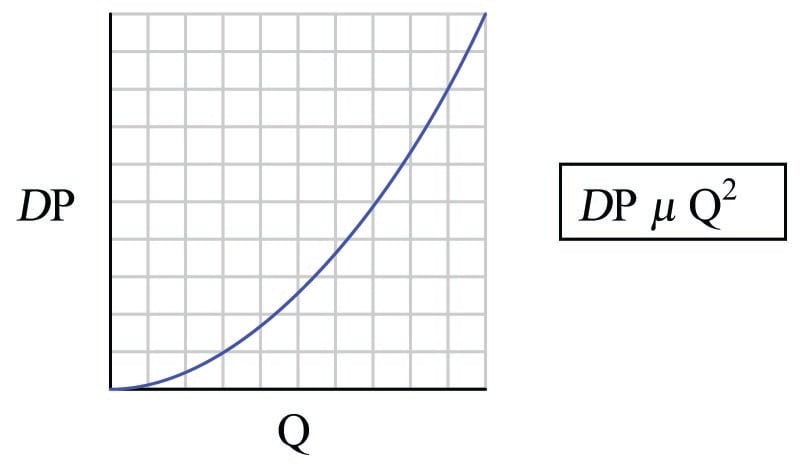
An unfortunate consequence of this quadratic relationship is that a pressure-sensing instrument connected to such a flow element will not directly sense flow rate. Instead, the pressure instrument will be sensing what is essentially the square of the flow rate. The instrument may register correctly at the 0% and 100% range points if correctly calibrated for the flow element it connects to, but it will fail to register linearly in between. Any indicator, recorder, or controller connected to the pressure-sensing instrument will likewise register incorrectly at any point between 0% and 100% of range, because the pressure signal is not a direct representation of flow rate.
In order that we may have indicators, recorders, and controllers that actually do register linearly with flow rate, we must mathematically “condition” or “characterize” the pressure signal sensed by the differential pressure instrument. Since the mathematical function inherent to the flow element is quadratic (square), the proper conditioning for the signal must be the inverse of that: square root. Just as taking the square-root of the square of a number yields the original number, taking the square-root of the differential pressure signal – which is itself a function of flow squared – yields a signal directly representing flow.
The traditional means of implementing the necessary signal characterization was to install a “square root” function relay between the transmitter and the flow indicator, as shown in the following diagram:
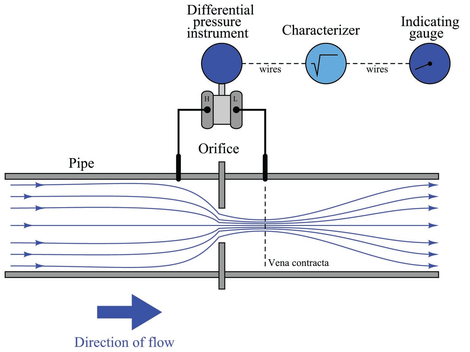
The modern solution to this problem is to incorporate square-root signal characterization either inside the transmitter or inside the receiving instrument (e.g. indicator, recorder, or controller). Either way, the square-root function must be implemented somewhere in the loop in order that flow may be accurately measured throughout the operating range.
In the days of pneumatic instrumentation, this square-root function was performed in a separate device called a square root extractor. The Foxboro model 557 (left) and Moore Products model 65 (right) pneumatic square root extractors are classic examples of this technology:
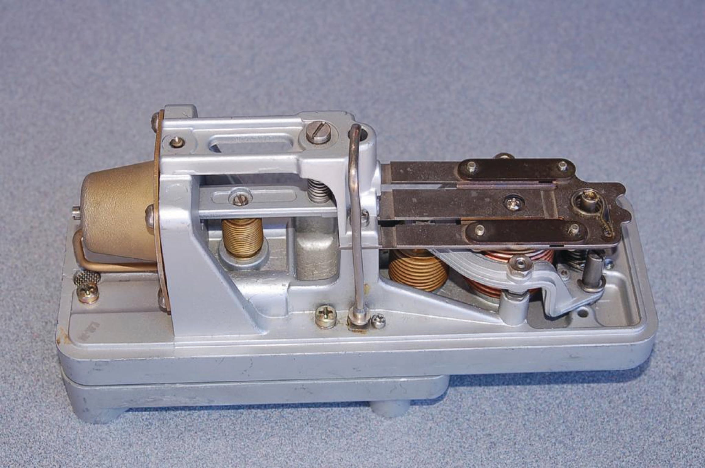
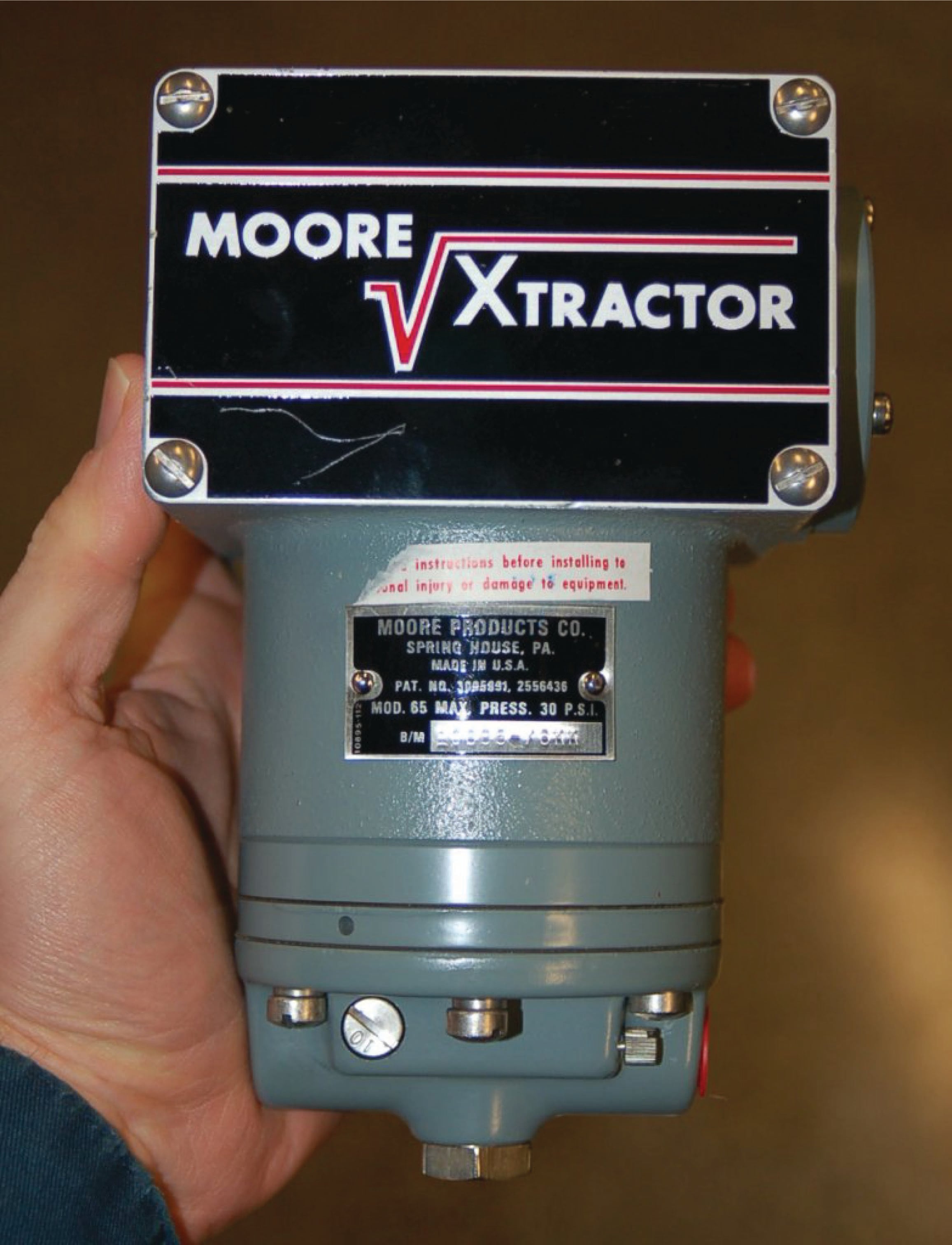
Pneumatic square root extraction relays approximated the square-root function by means of triangulated force or motion. In essence, they were trigonometric function relays, not square-root relays per se. However, for small angular motions, certain trigonometric functions were close enough to a square-root function that the relays were able to serve their purpose in characterizing the output signal of a pressure sensor to yield a signal representing flow rate.
The following table shows the ideal response of a pneumatic square root relay:
| Input signal | Input \% | Output \% & Output signal | |
|---|---|---|---|
| 3 PSI | 0\% | 0\% | 3 PSI |
| 4 PSI | 8.33\% | 28.87\% | 6.464 PSI |
| 5 PSI | 16.67\% | 40.82\% | 7.899 PSI |
| 6 PSI | 25\% | 50\% | 9 PSI |
| 7 PSI | 33.33\% | 57.74\% | 9.928 PSI |
| 8 PSI | 41.67\% | 64.55\% | 10.75 PSI |
| 9 PSI | 50\% | 70.71\% | 11.49 PSI |
| 10 PSI | 58.33\% | 76.38\% | 12.17 PSI |
| 11 PSI | 66.67\% | 81.65\% | 12.80 PSI |
| 12 PSI | 75\% | 86.60\% | 13.39 PSI |
| 13 PSI | 83.33\% | 91.29\% | 13.95 PSI |
| 14 PSI | 91.67\% | 95.74\% | 14.49 PSI |
| 15 PSI | 100\% | 100\% | 15 PSI |
As you can see from the table, the square-root relationship is most evident in comparing the input and output percentage values. For example, at an input signal pressure of 6 PSI (25%), the output signal percentage will be the square root of 25%, which is 50% (\(0.5 = \sqrt{0.25}\)) or 9 PSI as a pneumatic signal. At an input signal pressure of 10 PSI (58.33%), the output signal percentage will be 76.38%, because \(0.7638 = \sqrt{0.5833}\), yielding an output signal pressure of 12.17 PSI.
When graphed, the function of a square-root extractor is precisely opposite (inverted) of the quadratic function of a flow-sensing element such as an orifice plate, venturi, or pitot tube:
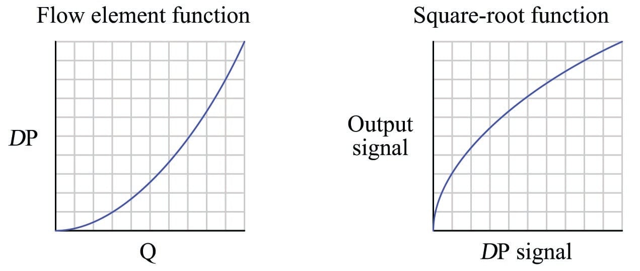
When cascaded – the square-root function placed immediately after the flow element’s “square” function – the result is an output signal that tracks linearly with flow rate (\(Q\)). An instrument connected to the square root relay’s signal will therefore register flow rate as it should.
Although analog electronic square-root relays have been built and used in industry for characterizing the output of 4-20 mA electronic transmitters, a far more common implementation of electronic square-root characterization occurs in DP transmitters designed with the square-root function built in. This way, no external relay device is necessary to characterize the DP transmitter’s signal into a flow rate signal:
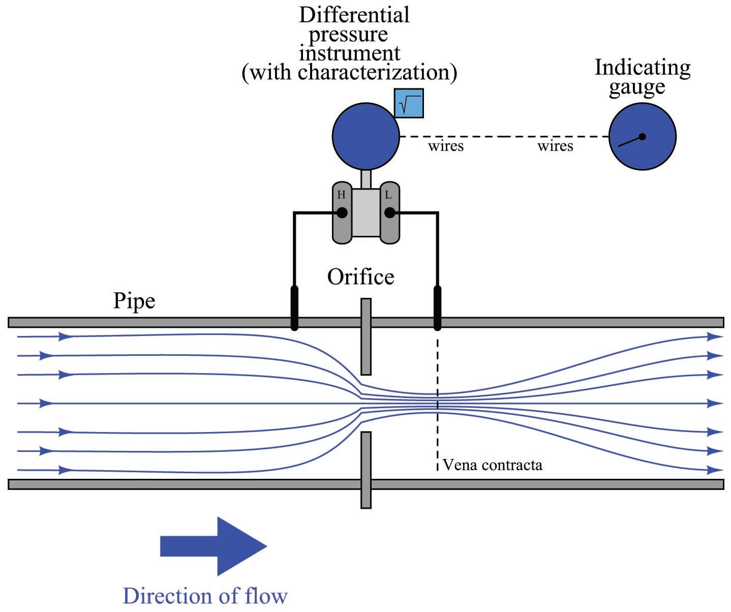
Using a characterized DP transmitter, any 4-20 mA sensing instrument connected to the transmitter’s output wires will directly interpret the signal as flow rate rather than as pressure. A calibration table for such a DP transmitter (with an input range of 0 to 150 inches water column) is shown here:
| $\Delta P$ | Input \% | Output \% = $\sqrt{\hbox Input \%}$ & Output signal | |
|---|---|---|---|
| 0 "W.C. | 0\% | 0\% | 4 mA |
| 37.5 "W.C. | 25\% | 50\% | 12 mA |
| 75 "W.C. | 50\% | 70.71\% | 15.31 mA |
| 112.5 "W.C. | 75\% | 86.60\% | 17.86 mA |
| 150 "W.C. | 100\% | 100\% | 20 mA |
Once again, we see how the square-root relationship is most evident in comparing the input and output percentages. Note how the percentages in this table precisely match the percentages in the pneumatic relay table: 0% input gives 0% output; 25% input gives 50% output, 50% input gives 70.71% output, etc.
An ingenious solution to the problem of square-root characterization, commonly seen in pneumatic flow-measurement systems where the DP transmitter lacks square-root characterization, is to use an indicating device with a square-root indicating scale. For example, the following photograph shows a 3-15 PSI “receiver gauge” designed to directly sense the output of a pneumatic DP transmitter:
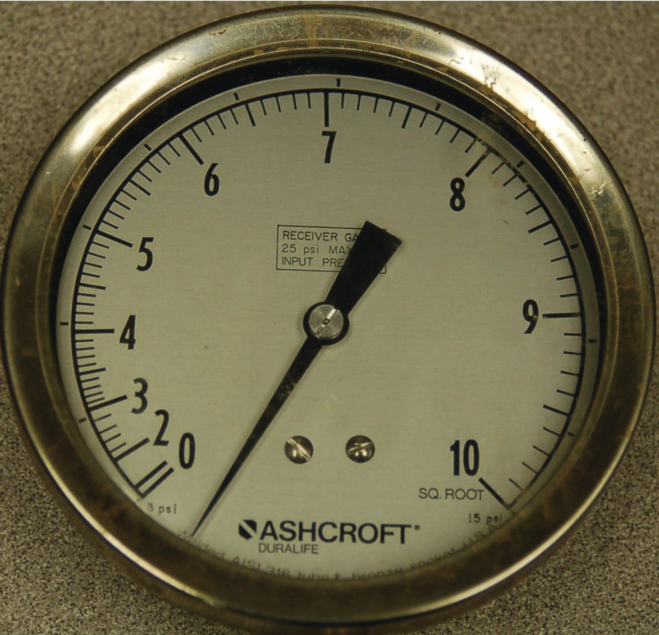
Note how the gauge mechanism responds directly and linearly to a 3-15 PSI input signal range (note the “3 PSI” and “15 PSI” labels in small print at the extremes of the scale, and the linearly-spaced marks around the outside of the scale arc representing 1 PSI each), but how the flow markings (0 through 10 on the inside of the scale arc) are spaced in a non-linear fashion.
An electronic variation on this theme is to draw a square-root scale on the face of a meter movement driven by the 4-20 mA output signal of an electronic DP transmitter:
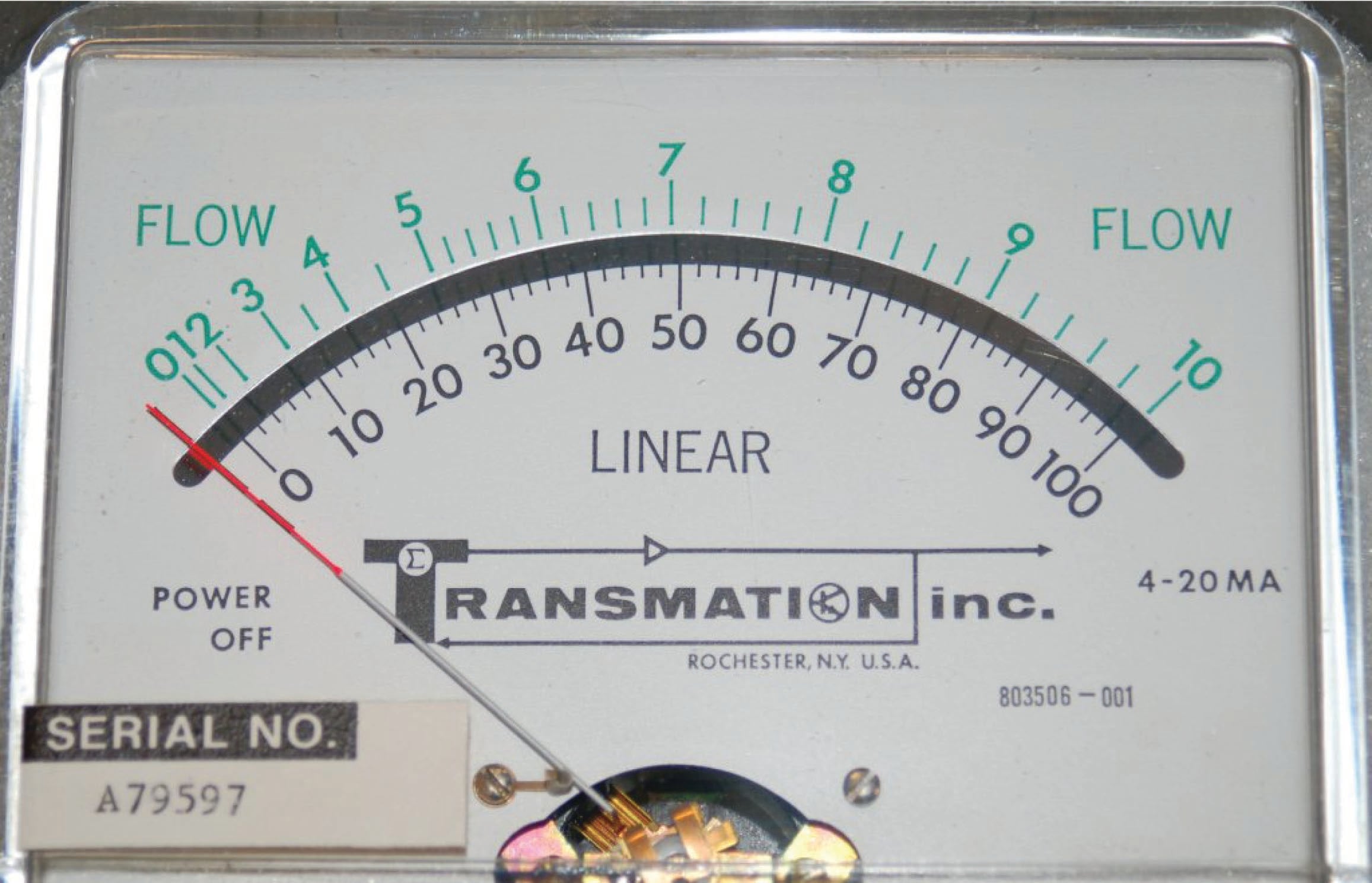
As with the square-root receiver gauge, the meter movement’s response to the transmitter signal is linear. Note the linear scale (drawn in black text labeled “LINEAR”) on the bottom and the corresponding square-root scale (in green text labeled “FLOW”) on the top. This makes it possible for a human operator to read the scale in terms of (characterized) flow units. Instead of using complicated mechanisms or circuitry to characterize the transmitter’s signal, a non-linear scale “performs the math” necessary to interpret flow.
A major disadvantage to the use of these non-linear indicator scales is that the transmitter signal itself remains un-characterized. Any other instrument receiving this un-characterized signal will either require its own square-root characterization or simply not interpret the signal in terms of flow at all. An un-characterized flow signal input to a process controller can cause loop instability at high flow rates, where small changes in actual flow rate result in huge changes in differential pressure sensed by the transmitter. A fair number of flow control loops operating without characterization have been installed in industrial applications (usually with square-root scales drawn on the face of the indicators, and square-root paper installed in chart recorders), but these loops are notorious for achieving good flow control at only one setpoint value. If the operator raises or lowers the setpoint value, the “gain” of the control loop changes thanks to the nonlinearities of the flow element, resulting in either under-responsive or over-responsive action from the controller.
Despite the limited practicality of non-linear indicating scales, they hold significant value as teaching tools. Closely examine the scales of both the receiver gauge and the 4-20 mA indicating meter, comparing the linear and square-root values at common points on each scale. A couple of examples are highlighted on the electric meter’s scale:
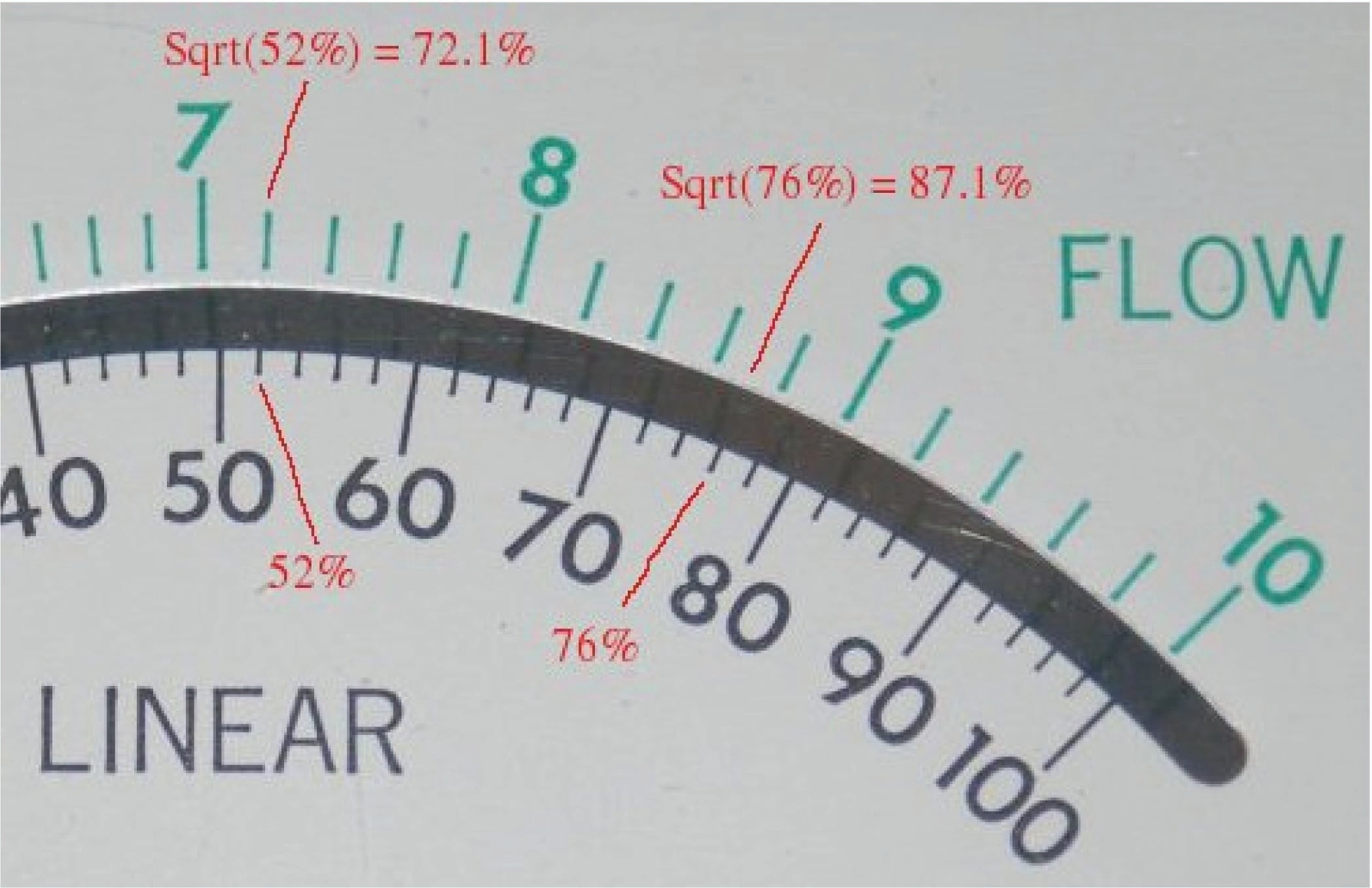
A few correlations between the linear and square-root scales of either the pneumatic receiver gauge or the electric indicating meter verify the fact that the square-root function is encoded in the spacing of the numbers on each instrument’s non-linear scale.
Another valuable lesson we may take from the faces of these indicating instruments is how uncertain the flow measurement becomes at the low end of the scale. Note how for each indicating instrument (both the receiver gauge and the meter movement), the square-root scale is “compressed” at the low end, to the point where it becomes impossible to interpret fine increments of flow at that end of the scale. At the high end of each scale, it’s a different situation entirely: the numbers are spaced so far apart that it’s easy to read fine distinctions in flow values (e.g. 94% flow versus 95% flow). However, the scale is so crowded at the low end that it’s really impossible to clearly distinguish two different flow values such as 4% from 5%.
This “crowding” is not just an artifact of a visual scale; it is a reflection of a fundamental limitation in measurement certainty with this type of flow measurement. The amount of differential pressure separating different low-range values of flow for a flow element is so little, even small amounts of pressure-measurement error equate to large amounts of flow-measurement error. In other words, it becomes more and more difficult to precisely interpret flow rate as the flow rate decreases toward the low end of the scale. The “crowding” we see on these indicator’s square-root scales is a visual reflection of this fundamental problem: even a small error in interpreting the pointer’s position at the low end of the scale can yield major errors in flow interpretation.
A technical term used to quantify this problem is turndown. “Turndown” refers to the ratio of high-range measurement to low-range measurement possible for an instrument while maintaining reasonable accuracy. For pressure-based flowmeters, which must deal with the non-linearities of Bernoulli’s Equation, the practical turndown is often no more than 3 to 1 (3:1). This means a flowmeter ranged for 0 to 300 GPM might only read with reasonable accurately down to a flow of 100 GPM. Below that, the accuracy becomes so poor that the measurement is almost useless. Advances in DP transmitter technology have pushed this ratio further, perhaps as far as 10:1 for certain installations. However, the fundamental problem is not transmitter resolution, but rather the nonlinearity of the flow element itself. This means any source of pressure-measurement error – whether originating in the transmitter’s pressure sensor or not – compromises our ability to accurately measure flow at low rates. Even with a perfectly calibrated transmitter, errors resulting from wear of the flow element (e.g. a dulled edge on an orifice plate) or from uneven liquid columns in the impulse tubes connecting the transmitter to the element, will cause large flow-measurement errors at the low end of the instrument’s range where the flow element produces only small differential pressures. Everyone involved with the technical details of flow measurement needs to understand this fact: the fundamental problem of limited turndown is grounded in the physics of turbulent flow and potential/kinetic energy exchange for these flow elements. Technological improvements will help, but they cannot overcome the limitations imposed by physics. If better turndown is required for a particular flow-measurement application, an entirely different flowmeter technology should be considered.
Orifice plates
Of all the pressure-based flow elements in existence, the most common is the orifice plate. This is simply a metal plate with a hole in the middle for fluid to flow through. Orifice plates are typically sandwiched between two flanges of a pipe joint, allowing for easy installation and removal:
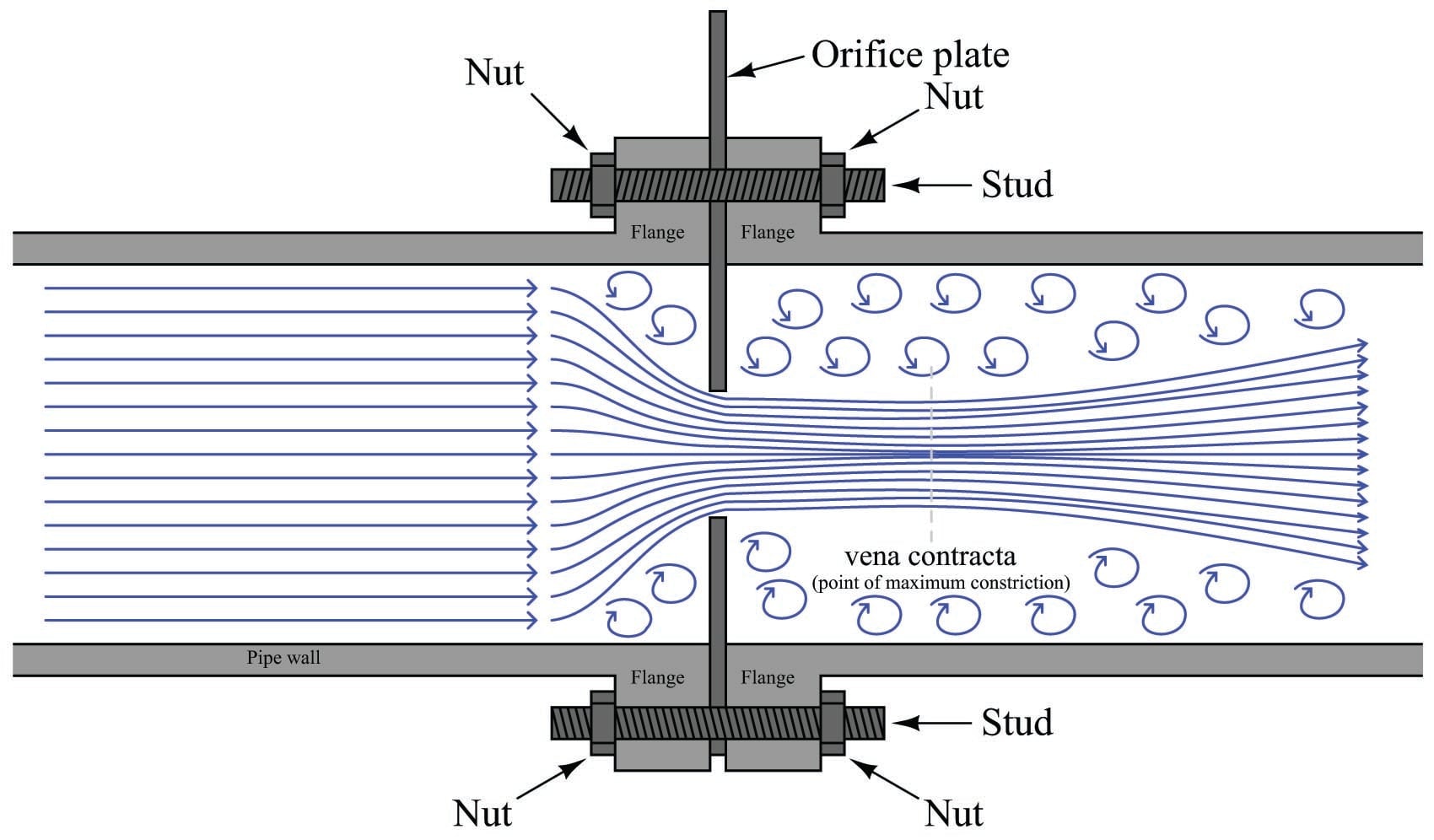
The point where the fluid flow profile constricts to a minimum cross-sectional area after flowing through the orifice is called the vena contracta, and it is the area of minimum fluid pressure. The vena contracta corresponds to the narrow throat of a venturi tube. The precise location of the vena contracta for an orifice plate installation will vary with flow rate, and also with the beta ratio (\(\beta\)) of the orifice plate, defined as the ratio of bore diameter (\(d\)) to inside pipe diameter (\(D\)):
\[\beta = {d \over D}\]
The simplest design of orifice plate is the square-edged, concentric orifice. This type of orifice plate is manufactured by machining a precise, straight hole in the middle of a thin metal plate. Looking at a side view of a square-edged concentric orifice plate reveals sharp edges (90\(^{o}\) corners) at the hole:
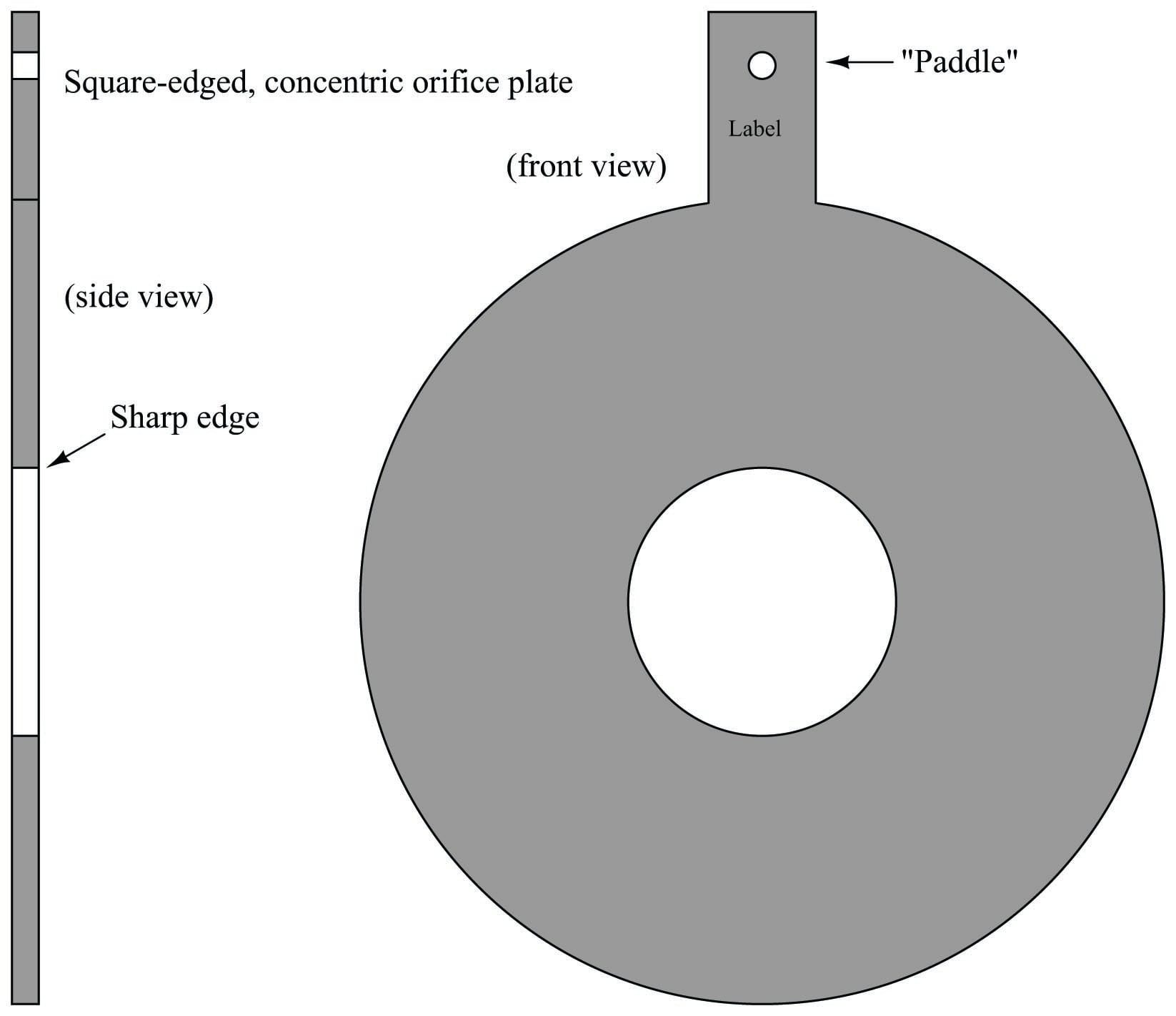
Square-edged orifice plates may be installed in either direction, since the orifice plate “appears” exactly the same from either direction of fluid approach. In fact, this allows square-edged orifice plates to be used for measuring bidirectional flow rates (where the fluid flow direction reverses itself from time to time). A text label printed on the “paddle” of any orifice plate customarily identifies the upstream side of that plate, but in the case of the square-edged orifice plate it does not matter.
The purpose of having a square edge on the hole in an orifice plate is to minimize contact with the fast-moving moving fluid stream going through the hole. Ideally, this edge will be knife-sharp. If the orifice plate is relatively thick (1/8 or an inch or more), it may be necessary to bevel the downstream side of the hole to further minimize contact with the fluid stream:
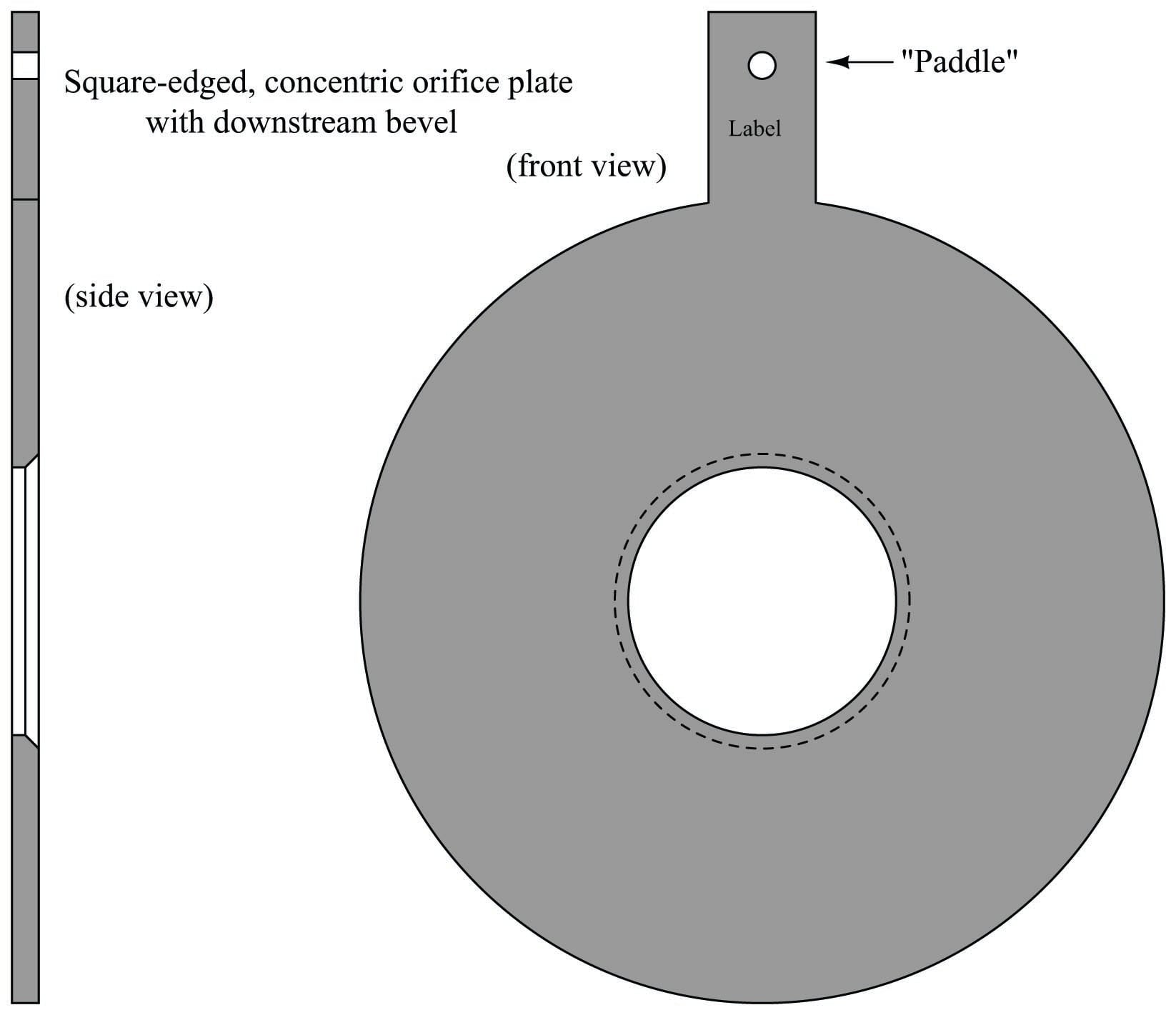
Looking at the side-view of this orifice plate, the intended direction of flow is left-to-right, with the sharp edge facing the incoming fluid stream and the bevel providing a non-contact outlet for the fluid. Beveled orifice plates are obviously uni-directional, and must be installed with the paddle text facing upstream.
Other square-edged orifice plates exist to address conditions where gas bubbles or solid particles may be present in liquid flows, or where liquid droplets or solid particles may be present in gas flows. The first of this type is called the eccentric orifice plate, where the hole is located off-center to allow the undesired portions of the fluid to pass through the orifice rather than build up on the upstream face:
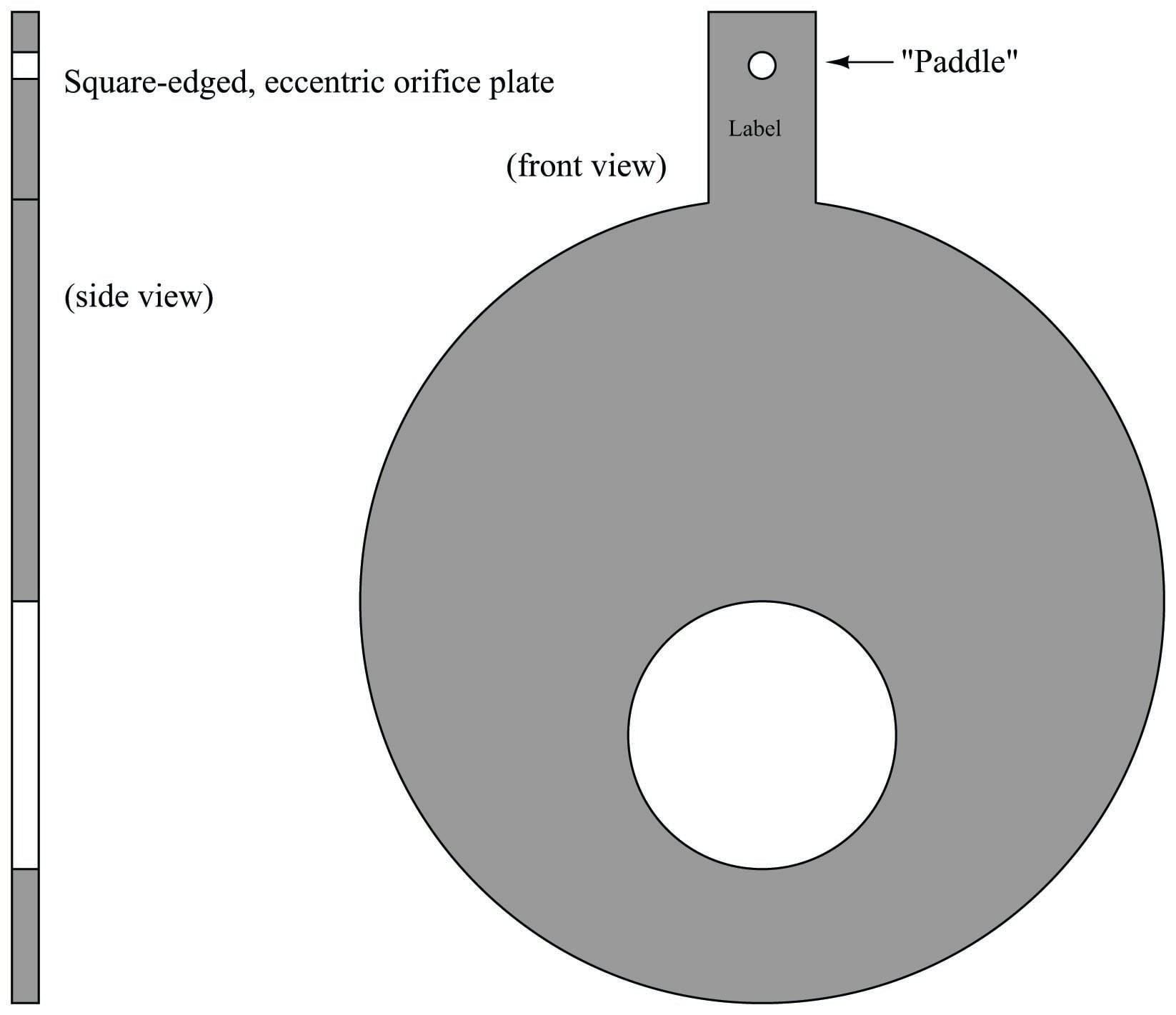
For gas flows, the hole should be offset downward, so any liquid droplets or solid particles may easily pass through. For liquid flows, the hole should be offset upward to allow gas bubbles to pass through and offset downward to allow heavy solids to pass through.
The second off-center orifice plate type is called the segmental orifice plate, where the hole is not circular but rather just a segment of a concentric circle:
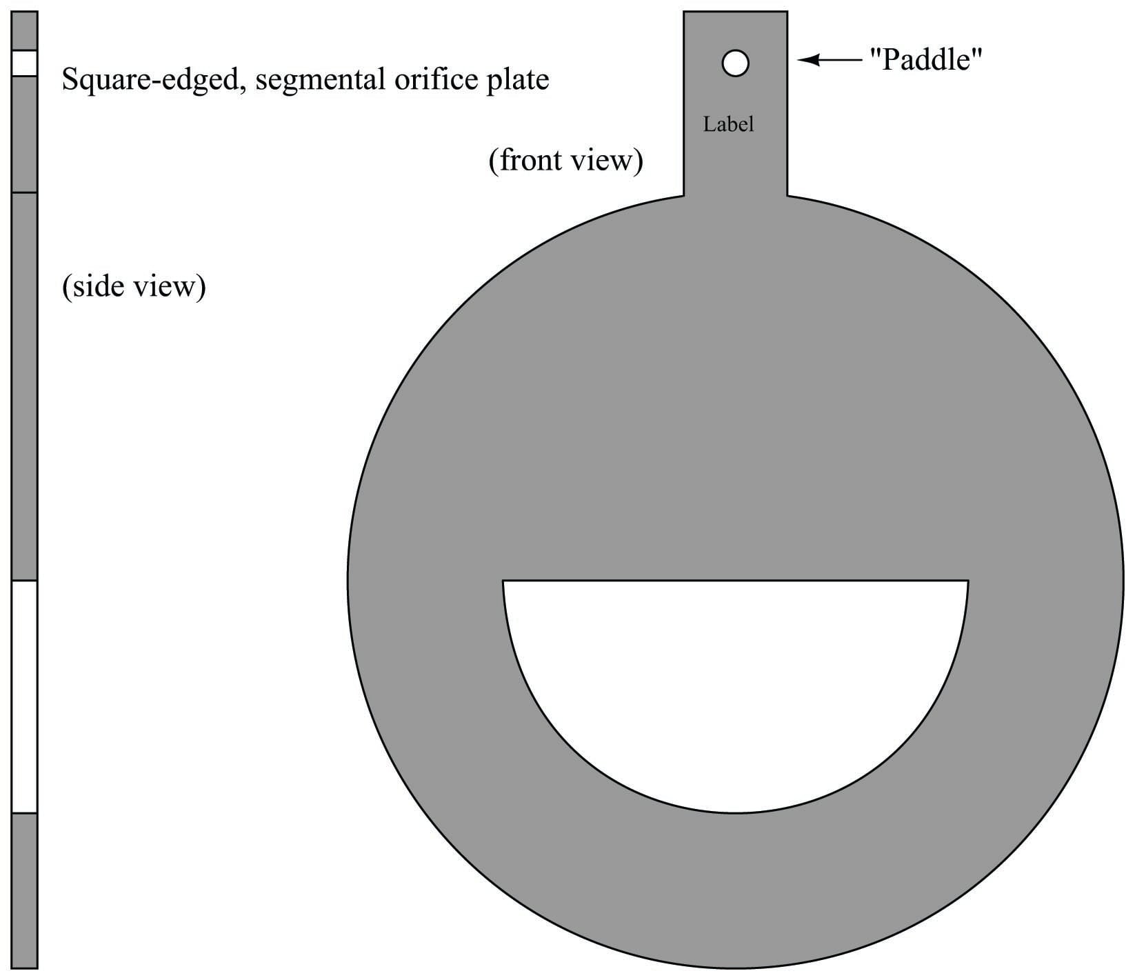
As with the eccentric orifice plate design, the segmental hole should be offset downward in gas flow applications and either upward or downward in liquid flow applications depending on the type of undesired material(s) in the flowstream.
An alternative to offsetting or re-shaping the bore hole of an orifice plate is to simply drill a small hole near the edge of the plate, flush with the inside diameter of the pipe, allowing undesired substances to pass through the plate rather than collect on the upstream side. If such a hole is oriented upward to pass vapor bubbles, it is called a vent hole. If the hole is oriented downward to pass liquid droplets or solids, it is called a drain hole. Vent and drain holes are useful when the concentration of these undesirable substances is not significant enough to warrant either an eccentric or segmental orifice:
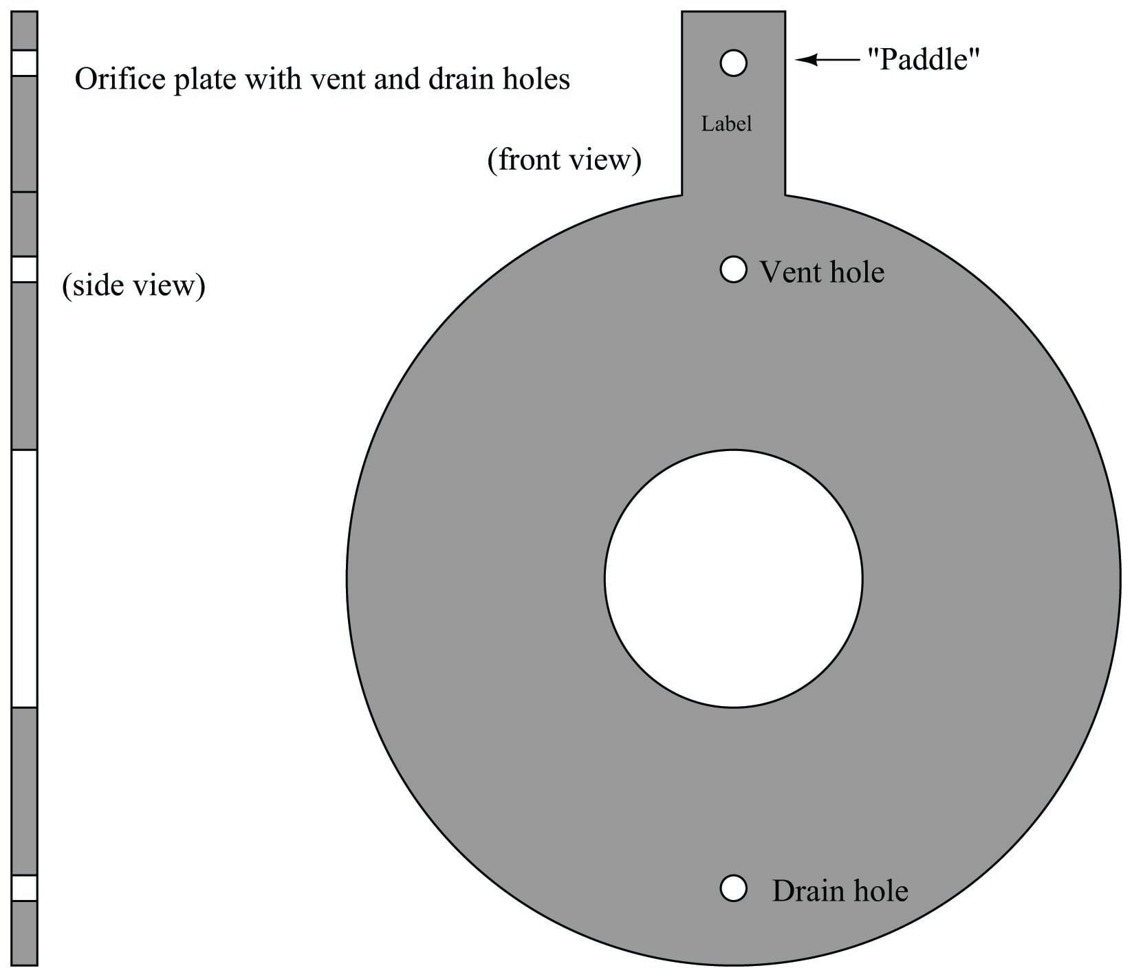
The addition of a vent or drain hole should have negligible impact on the performance of an orifice plate due to its small size relative to the main bore. If the quantity of undesirable material in the flowstream (bubbles, droplets, or solids) is excessive, an eccentric or segmental orifice plate might be a better choice.
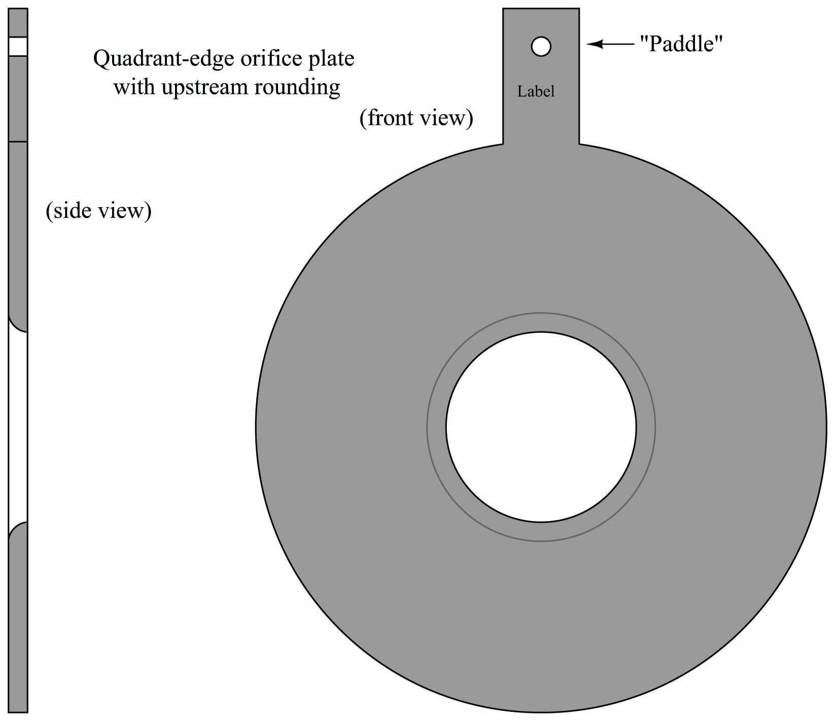
Some orifice plates employ non-square-edged holes for the purpose of improving performance at low Reynolds number values, where the effects of fluid viscosity are more apparent. These orifice plate types employ rounded- or conical-entrance holes in an effort to minimize the effects of fluid viscosity. Experiments have shown that decreased Reynolds number causes the flowstream to not contract as much when traveling through an orifice, thus limiting fluid acceleration and decreasing the amount of differential pressure produced by the orifice plate. However, experiments have also shown that decreased Reynolds number in a venturi-type flow element causes an increase in differential pressure due to the effects of friction against the entrance cone walls. By manufacturing an orifice plate in such a way that the hole exhibits “venturi-like” properties (i.e. a dull edge where the fast-moving fluid stream has more contact with the plate), these two effects tend to cancel each other, resulting in an orifice plate that maintains consistent accuracy at lower flow rates and/or higher viscosities than the simple square-edged orifice.
Two common non-square-edge orifice plate designs are the quadrant-edge and conical-entrance orifices. The quadrant-edge is shown first:
The conical-entrance orifice plate looks like a beveled square-edge orifice plate installed backwards, with flow entering the conical side and exiting the square-edged side:
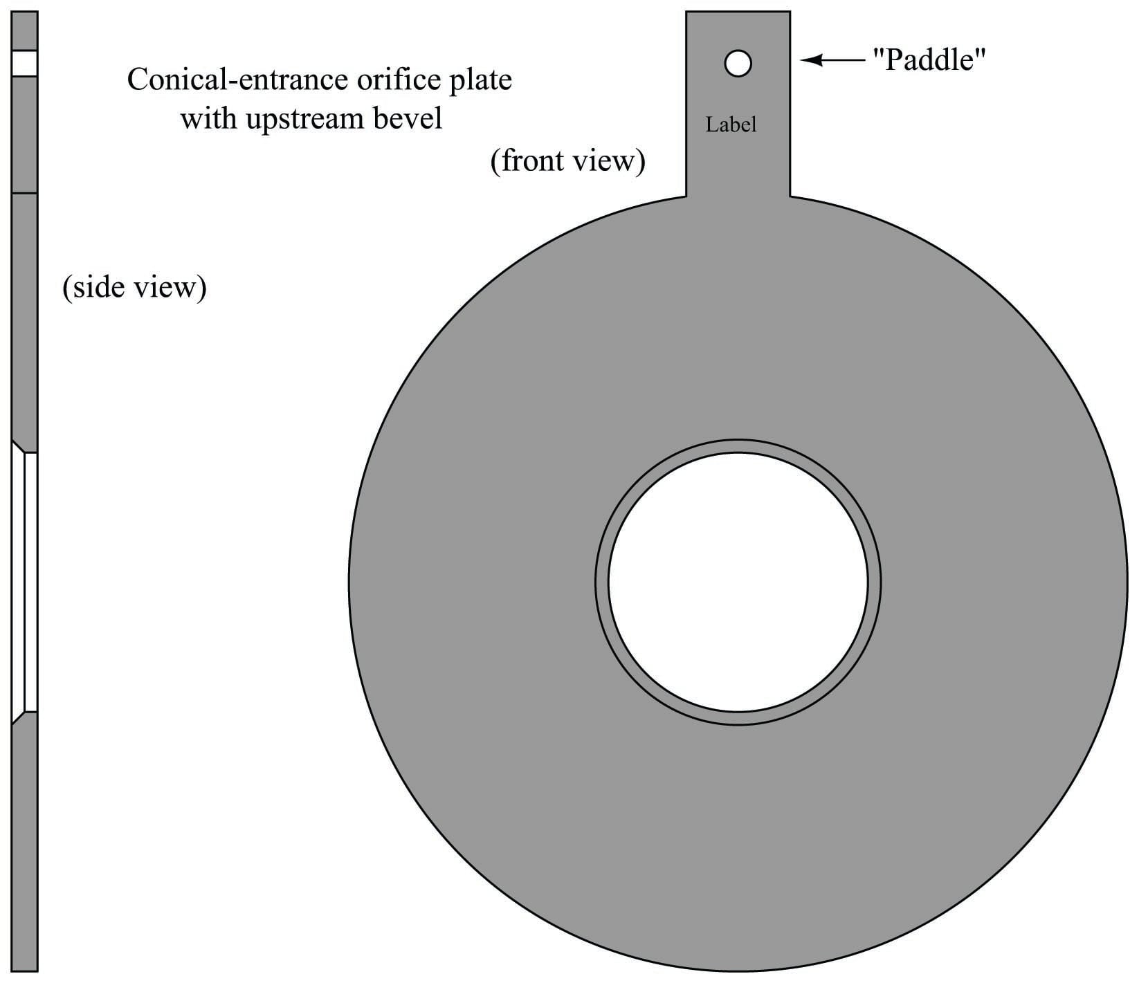
Here, is it vitally important to pay attention to the paddle’s text label. This is the only sure indication of which direction an orifice plate needs to be installed. One can easily imagine an instrument technician mistaking a conical-entrance orifice plate for a square-edged, beveled orifice plate and installing it backward!
Several standards exist for pressure tap locations. Ideally, the upstream pressure tap will detect fluid pressure at a point of minimum velocity, and the downstream tap will detect pressure at the vena contracta (maximum velocity). In reality, this ideal is never perfectly achieved. An overview of the most popular tap locations for orifice plates is shown in the following illustration:
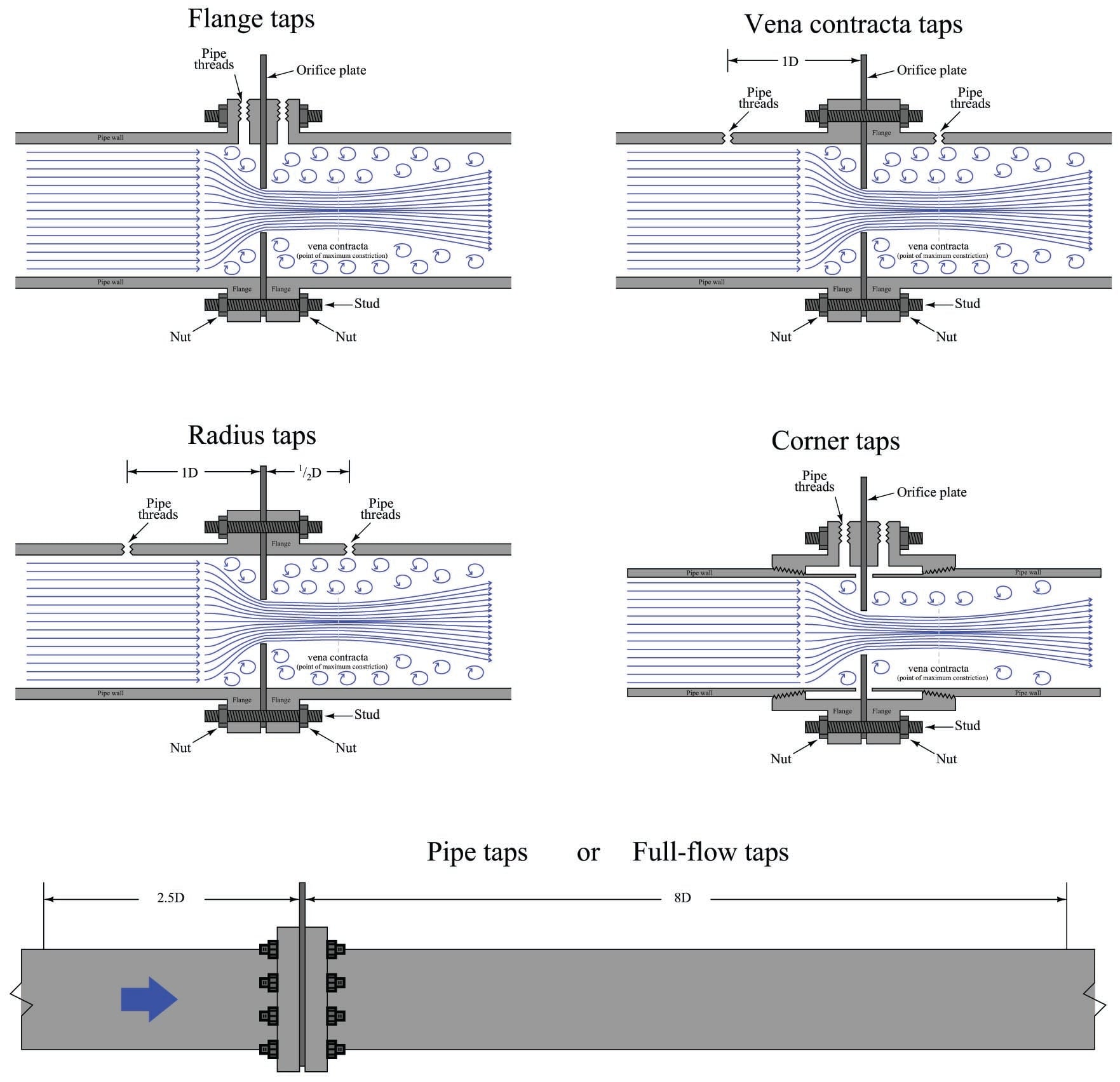
Flange taps are the most popular tap location for orifice meter runs on large pipes in the United States. Flanges may be manufactured with tap holes pre-drilled and finished before the flange is even welded to the pipe, making this a very convenient pressure tap configuration. Most of the other tap configurations require drilling into the pipe after installation, which is not only labor-intensive, but may possibly weaken the pipe at the locations of the tap holes.
Vena contracta taps offer the greatest differential pressure for any given flow rate, but require precise calculations to properly locate the downstream tap position. Radius taps are an approximation of vena contracta taps for large pipe sizes (one-half pipe diameter downstream for the low-pressure tap location). An unfortunate characteristic of both these taps is the requirement of drilling through the pipe wall. Not only does this weaken the pipe, but the practical necessity of drilling the tap holes in the installed location rather than in a controlled manufacturing environment means there is considerable room for installation error.
Corner taps must be used on small pipe diameters where the vena contracta is so close to the downstream face of the orifice plate that a downstream flange tap would sense pressure in the highly turbulent region (too far downstream). Corner taps obviously require special (i.e. expensive) flange fittings, which is why they tend to be used only when necessary.
Care should be taken to avoid measuring downstream pressure in the highly turbulent region following the vena contracta. This is why the pipe tap (also known as full-flow tap) standard calls for a downstream tap location eight pipe diameters away from the orifice: to give the flow stream room to stabilize for more consistent pressure readings.
Wherever the taps are located, it is vitally important that the tap holes be completely flush with the inside wall of the pipe or flange. Even the smallest recess or burr left from drilling will cause measurement errors, which is why tap holes are best drilled in a controlled manufacturing environment rather that at the installation site where the task will likely be performed by non-experts.
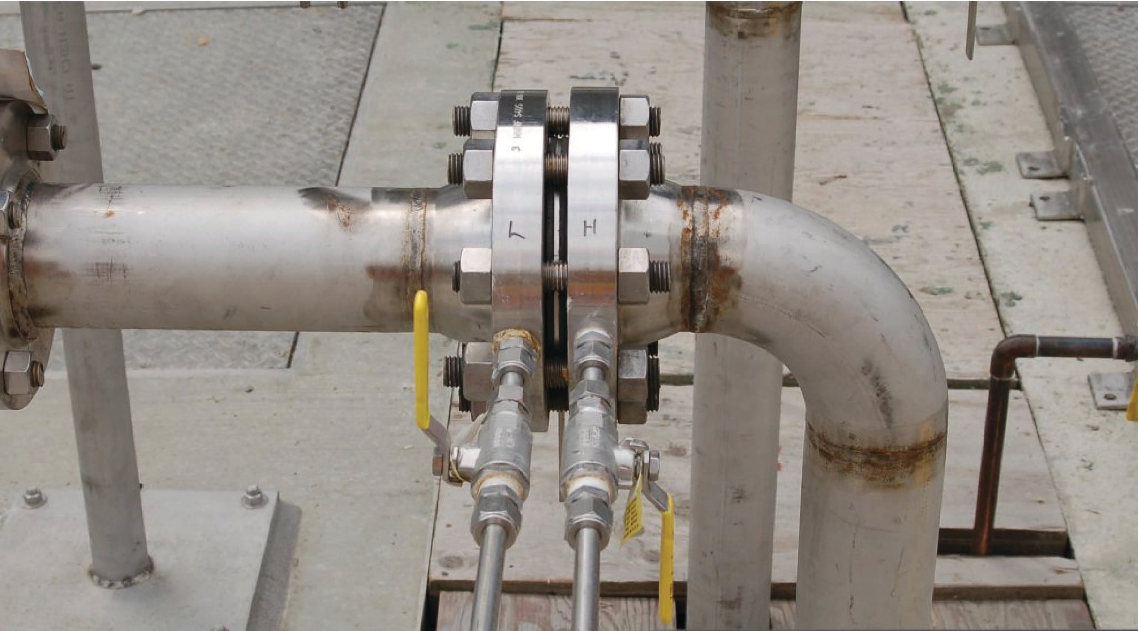
A photograph of an orifice plate used to measure the flow of natural gas to a large turbine engine is shown here, with a Rosemount model 3051 differential pressure transmitter sensing the pressure drop generated by the orifice:
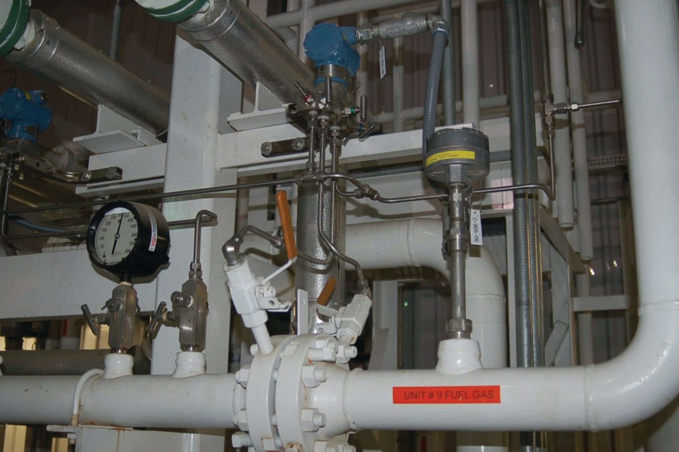
Flange taps are used in this orifice installation, with the taps and pressure transmitter located above the pipe centerline to avoid picking up any liquid droplets that may pass through the pipe. The direction of gas flow in this particular installation is from left to right, making the left-hand pressure tap the “high pressure” side and the right-hand pressure tap the “low pressure” side.
As you can see by the pressure gauge’s indication in the photograph, the static line pressure of the natural gas inside the pipe is over 300 PSI. The amount of pressure drop generated by the orifice plate at full flow, however, is likely only a few PSI (100 inches water column is typical for many orifice plate installations). This is why we must use a differential pressure transmitter to measure the orifice plate’s pressure drop: only a DP transmitter will sense the difference in pressure across the orifice while rejecting the static (common-mode) line pressure inside the pipe.
A photograph of another orifice plate with flange taps appears here, shown on a vertical pipe. In this example, the pipe and flanges are formed of acrylic (transparent plastic):
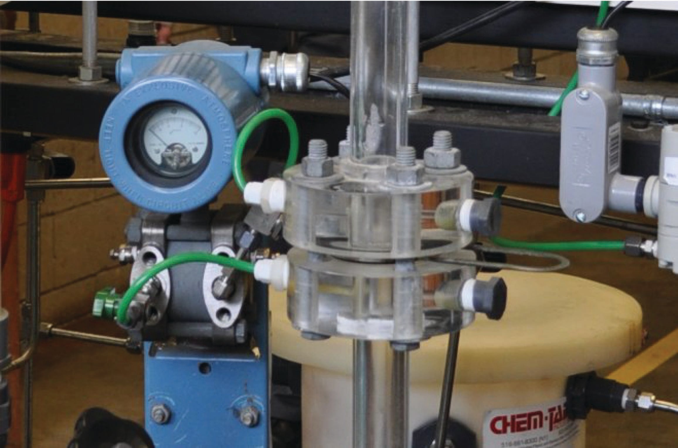
As is customary with orifice plates mounted in vertical pipes, the direction of flow is upward (from bottom to top), making the bottom tap the “high pressure” side and the top tap the “low pressure” side. Since this is a liquid application, the transmitter is located below the taps in order to avoid collecting bubbles of air or other gases in the impulse lines.
This particular orifice and flow transmitter (Rosemount model 1151) is used on a process “trainer” unit at Brazosport College in Lake Jackson, Texas. The transparent flanges, pipes, and process vessels make it easier for students to visualize the fluid motion.
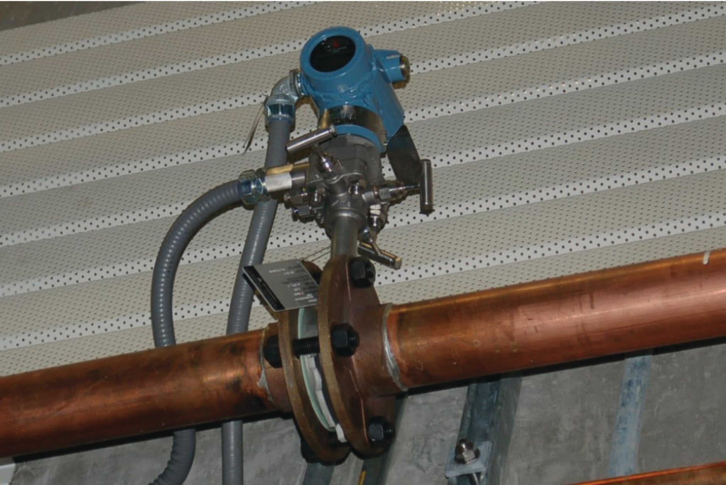
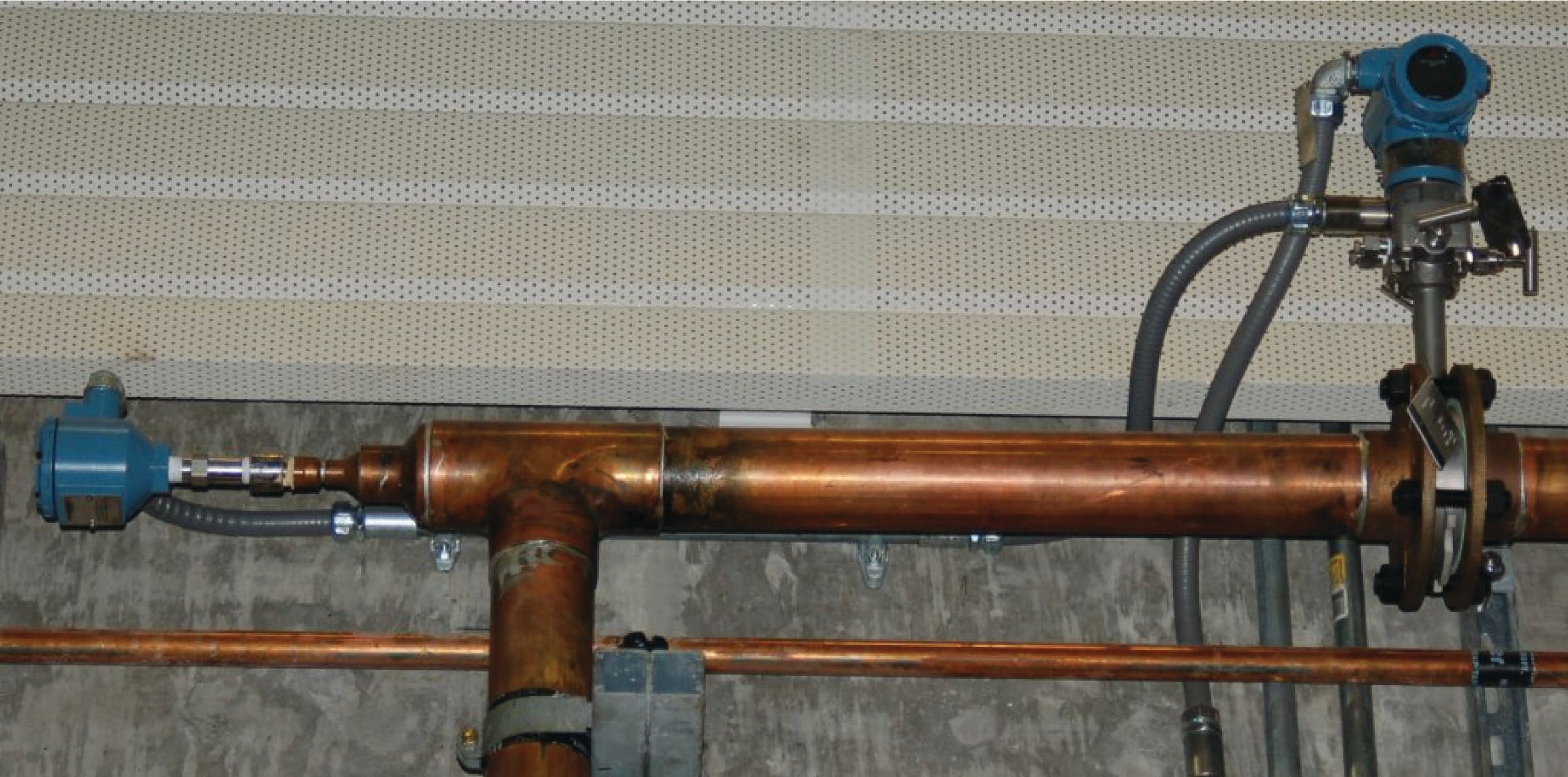
For relatively low flow rates, an alternative arrangement is the integral orifice plate. This is where a small orifice plate directly attaches to the differential pressure-sensing element, eliminating the need for impulse lines. A photograph of an integral orifice plate and transmitter is shown here, in an application measuring the flow of purified oxygen gas through a copper pipe:
Even smaller integral orifices exist for the measurement of very low flow rates, another type of integral orifice is available. This style uses the pass-through nature of a typical differential pressure transmitter’s capsule flanges to advantage. Note the paths of fluid flow, as well as the unusual orientation of the three-valve manifold, in these two example illustrations:
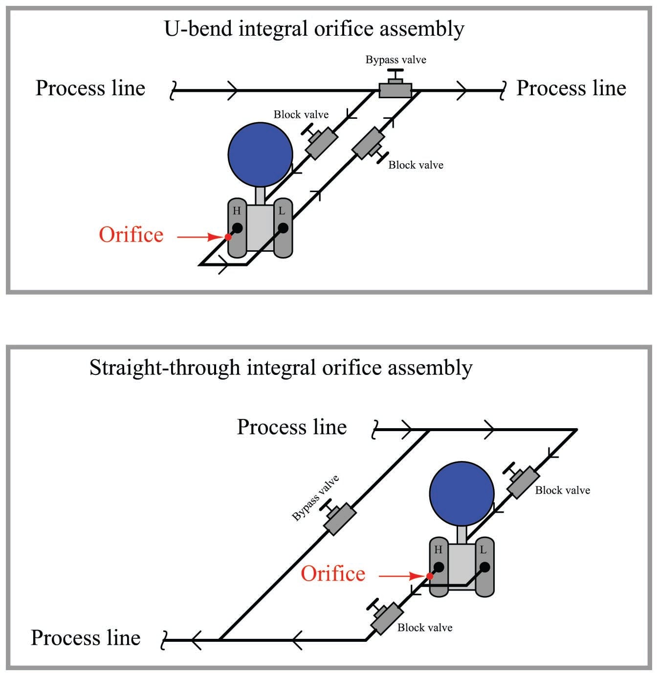
In both examples, the third hand valve serves the purpose of bypassing process fluid flow rather than equalizing both ports of the differential pressure transmitter. Process fluid actually flows through at least one chamber of the DP transmitter’s body. Clearly, this kind of integral orifice plate is practical only for very low rates of flow, typically where the process flow line is no larger than the size of the pressure ports on the transmitter’s body.
The task of properly sizing an orifice plate for any given application is complex enough to recommend the use of special orifice sizing computer software provided by orifice plate manufacturers. There are a number of factors to consider in orifice plate sizing, and these software packages account for all of them. Best of all, the software provided by manufacturers is often linked to data for that manufacturer’s product line, helping to assure installed results in close agreement with predictions.
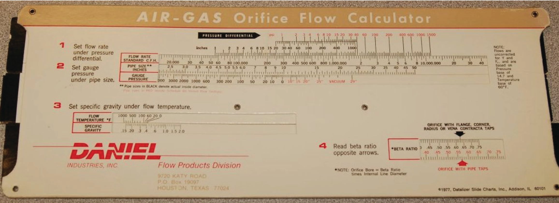
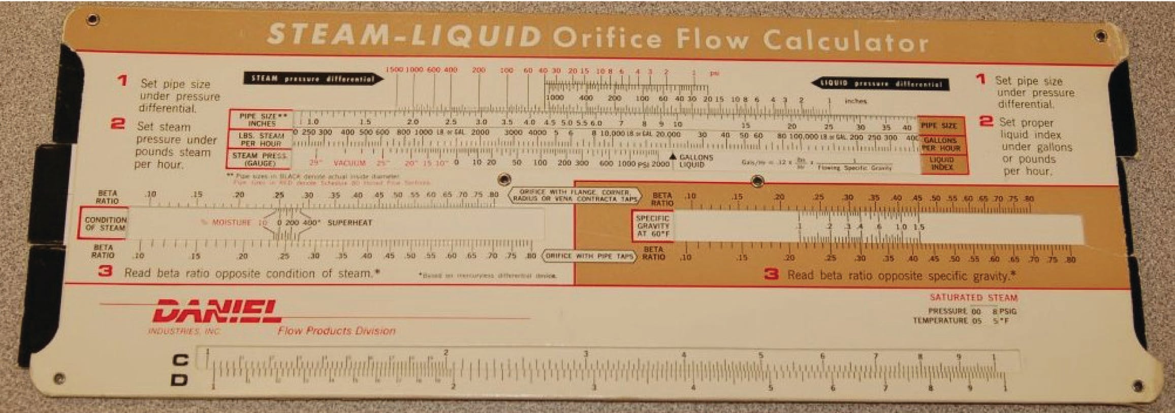
In the days before ubiquitous personal computers and the Internet, some orifice plate manufacturers provided customers with paper “slide rule” calculators to help them select appropriate orifice plate sizes from known process parameters. The following photographs show the front and back sides of one such slide rule:
Other differential producers
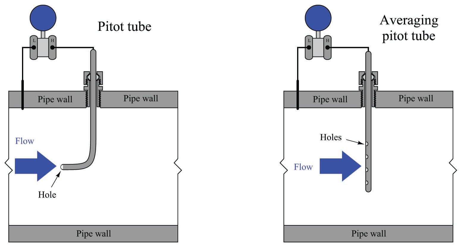
Other pressure-based flow elements exist as alternatives to the orifice plate. The Pitot tube, for example, senses pressure as the fluid stagnates (comes to a complete stop) against the open end of a forward-facing tube. A shortcoming of the classic single-tube Pitot assembly is sensitivity to fluid velocity at just one point in the pipe, so a more common form of Pitot tube seen in industry is the averaging Pitot tube consisting of several stagnation holes sensing velocity at multiple points across the width of the flow:
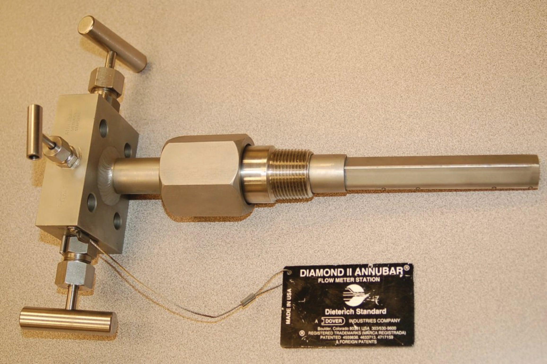
A variation on the latter theme is the Annubar flow element, a trade name of the Dieterich Standard corporation. An “Annubar” is an averaging pitot tube consolidating high and low pressure-sensing ports in a single probe assembly:
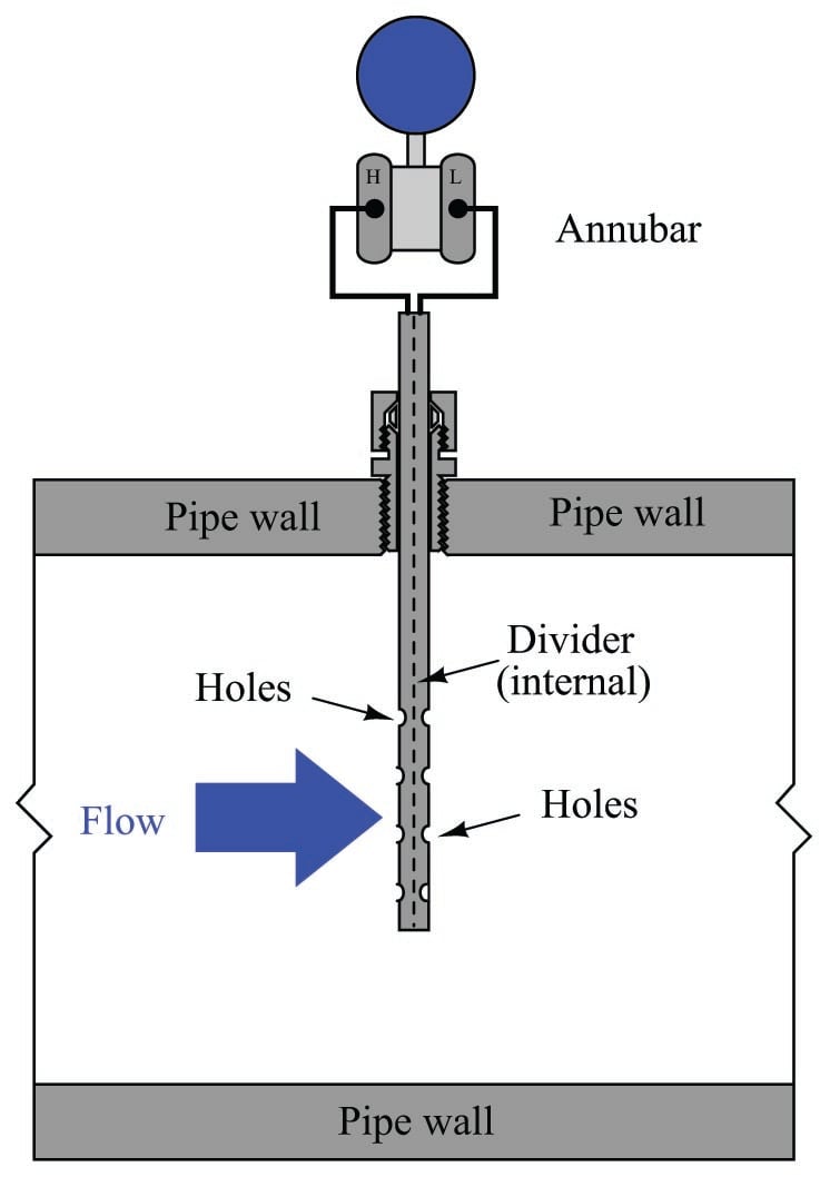
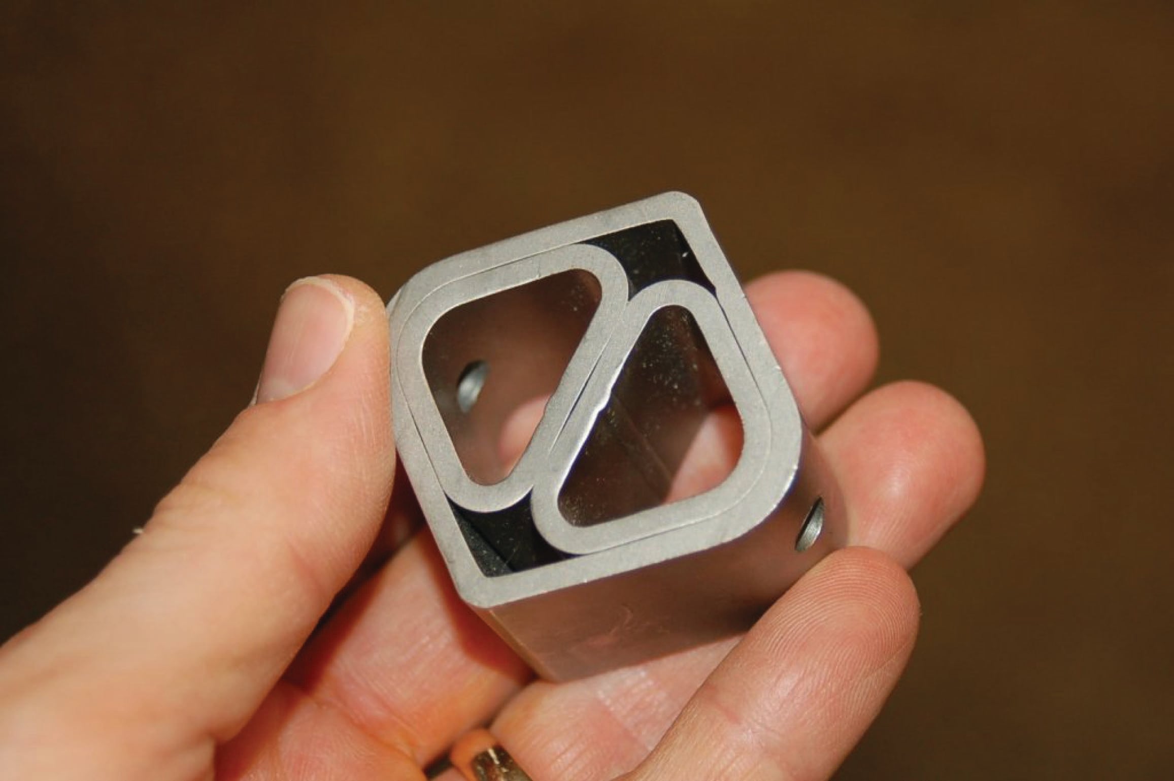
What appears at first glance to be a single, square-shaped tube inserted into the pipe is actually a double-ported tube with holes on both the upstream and downstream edges:
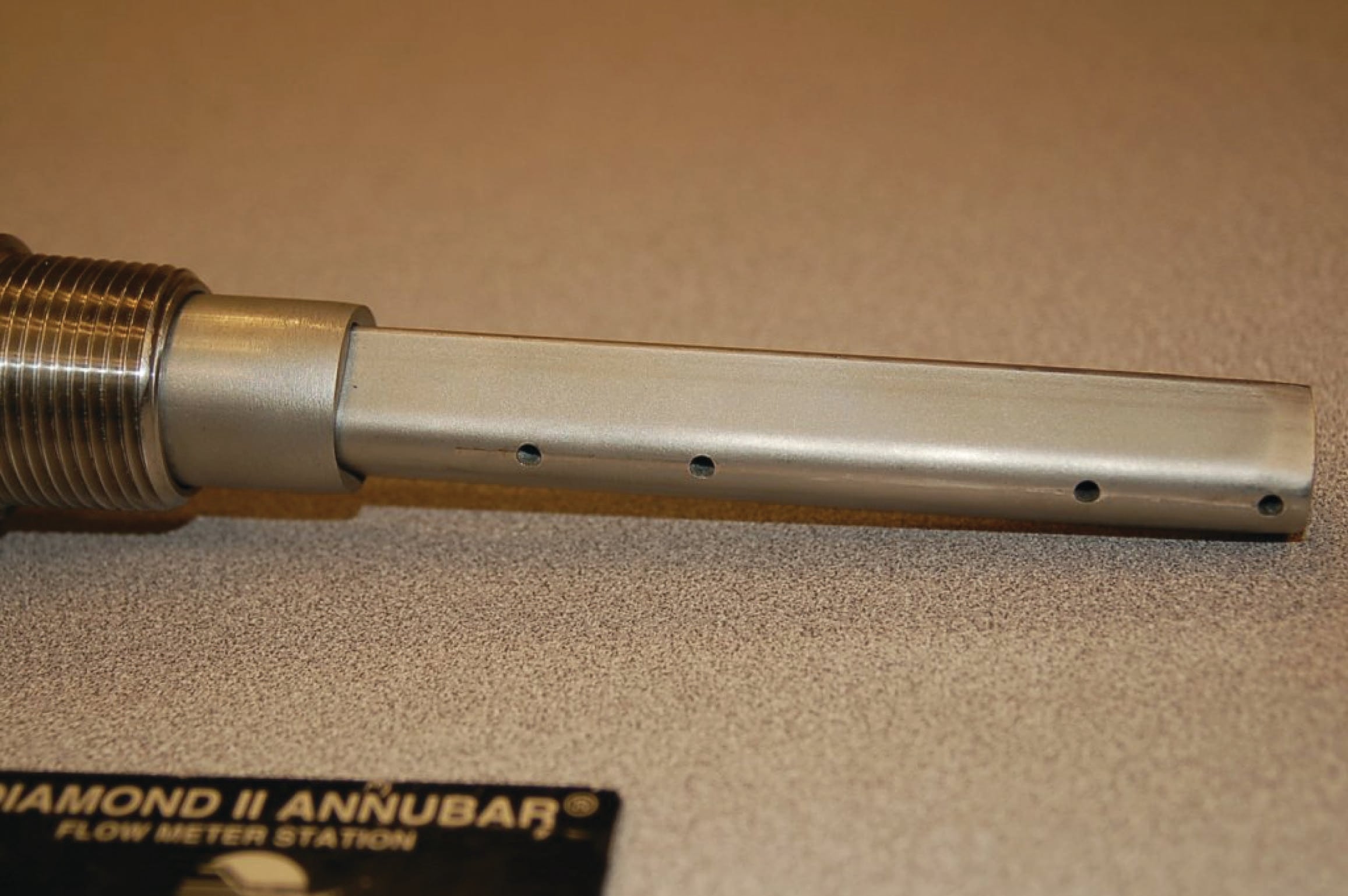
A section of Annubar tube clearly shows the porting and dual chambers, designed to bring upstream (stagnation) and downstream pressures out of the pipe to a differential pressure-sensing instrument:
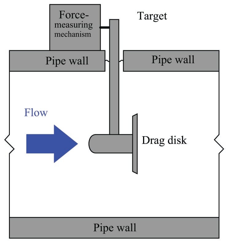
A less sophisticated realization of the stagnation principle is the target flow sensor, consisting of a blunt “paddle” (or “drag disk”) inserted into the flowstream. The force exerted on this paddle by the moving fluid is sensed by a special transmitter mechanism, which then outputs a signal corresponding to flow rate (proportional to the square of fluid velocity, just like an orifice plate):
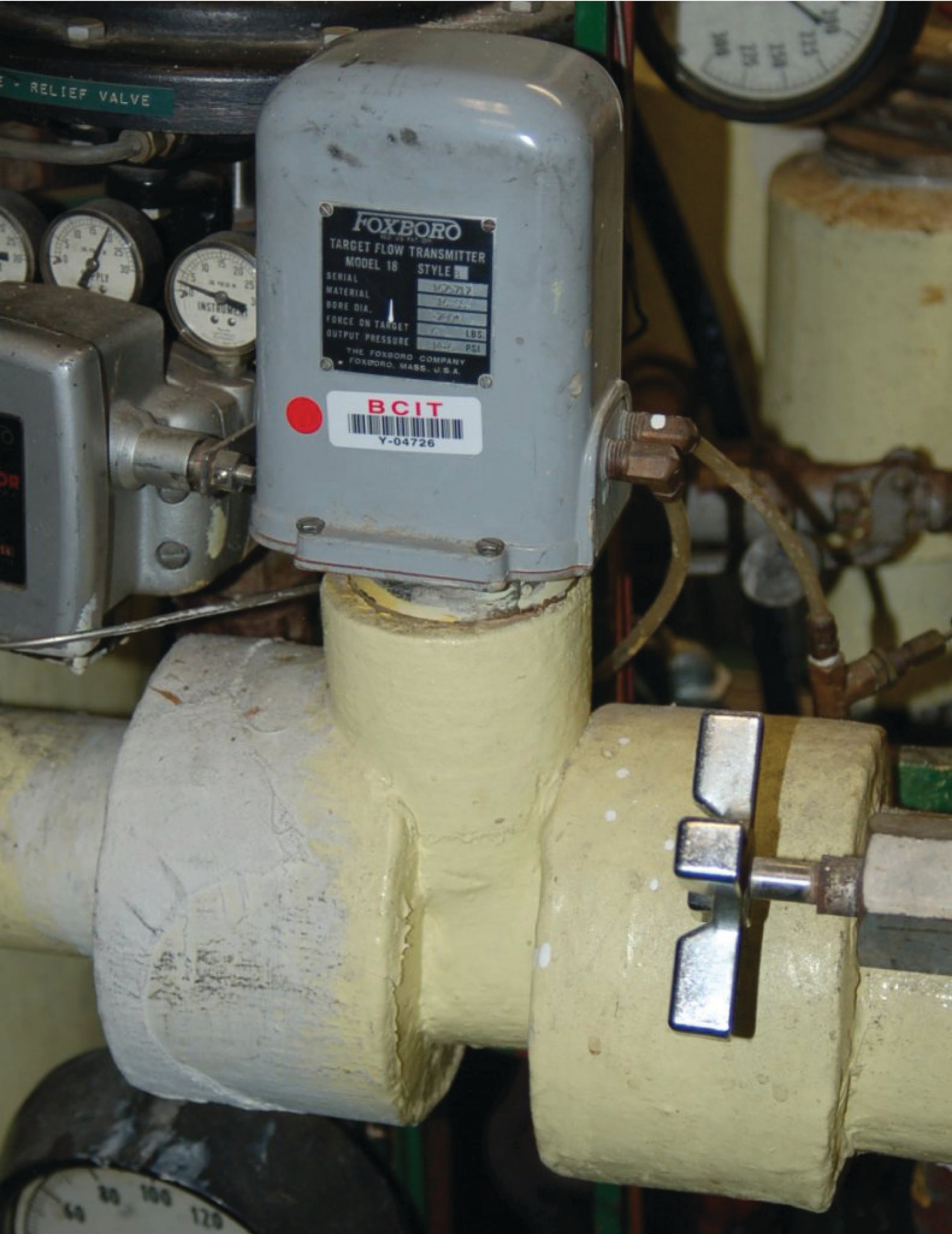
The following photograph shows a Foxboro model 18 target flow transmitter installed on a line conveying liquid wood pulp:
The classic venturi tube pioneered by Clemens Herschel in 1887 has been adapted in a variety of forms broadly classified as flow tubes. All flow tubes work on the same principle: developing a differential pressure by channeling fluid flow from a wide tube to a narrow tube. The differ from the classic venturi only in construction details, the most significant detail being a significantly shorter length than the classic venturi tube. Examples of flow tube designs include the Dall tube, Lo-Loss flow tube, Gentile or Bethlehem flow tube, and the B.I.F. Universal Venturi.
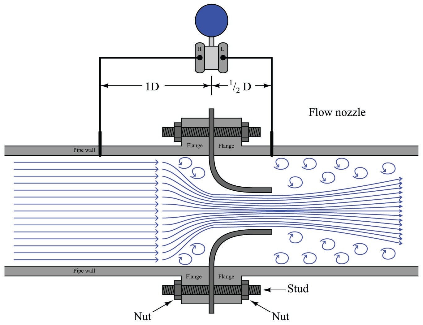
Another variation on the venturi theme is called a flow nozzle, designed to be clamped between the faces of two pipe flanges in a manner similar to an orifice plate. The goal here is to achieve simplicity of installation approximating that of an orifice plate while improving performance (less permanent pressure loss) over orifice plates:
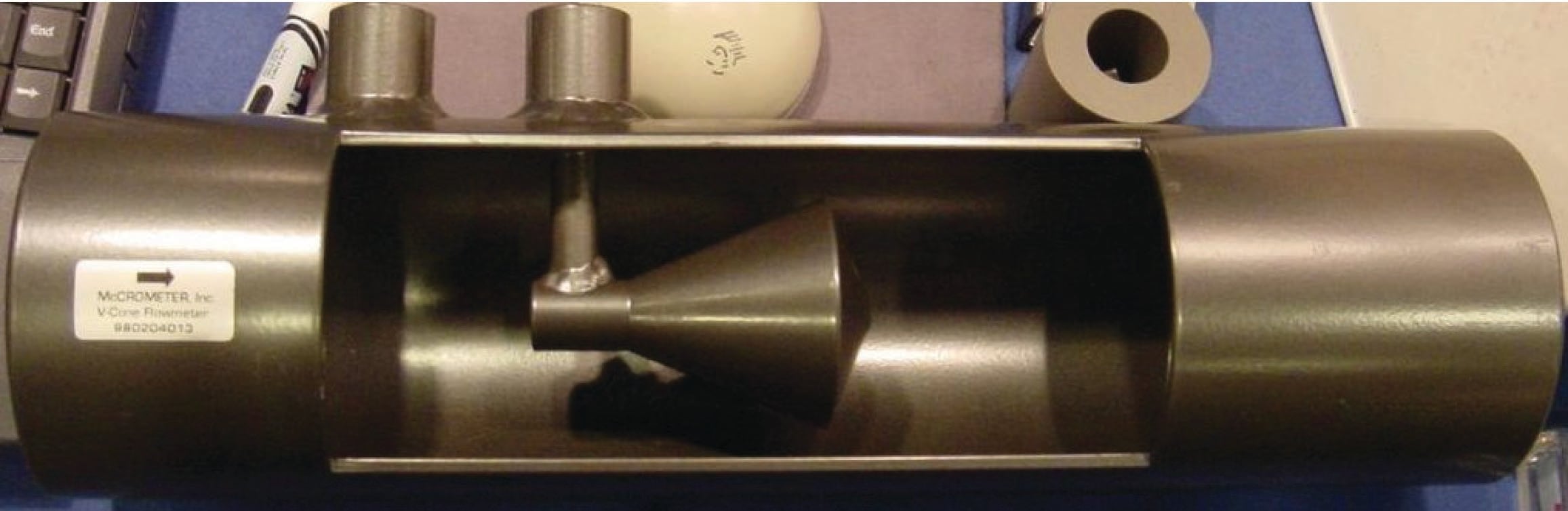
Two more variations on the venturi theme are the V-cone and Segmental wedge flow elements. The V-cone (or “venturi cone,” a trade name of the McCrometer division of the Danaher corporation) may be thought of as a venturi tube or orifice plate in reverse: instead of narrowing the tube’s diameter to cause fluid acceleration, fluid must flow around a cone-shaped obstruction placed in the middle of the tube. The tube’s effective area will be reduced by the presence of this cone, causing fluid to accelerate through the restriction just as it would through the throat of a classic venturi tube:
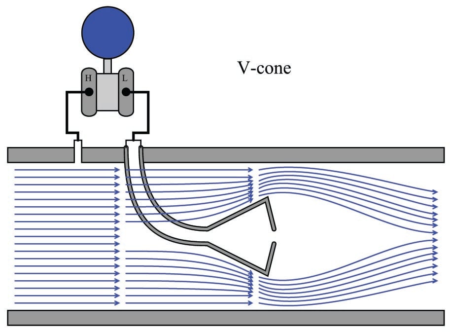
This cone is hollow, with a pressure-sensing port on the downstream side allowing for easy detection of fluid pressure near the vena contracta. Upstream pressure is sensed by another port in the pipe wall upstream of the cone. The following photograph shows a V-cone flow tube, cut away for demonstration purposes:
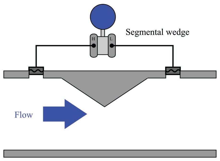
Segmental wedge elements are special pipe sections with wedge-shaped restrictions built in. These devices, albeit crude, are useful for measuring the flow rates of slurries, especially when pressure is sensed by the transmitter through remote-seal diaphragms (to eliminate the possibility of impulse tube plugging):
Finally, the lowly pipe elbow may be pressed into service as a flow-measuring element, since fluid turning a corner in the elbow experiences radial acceleration and therefore generates a differential pressure along the axis of acceleration:
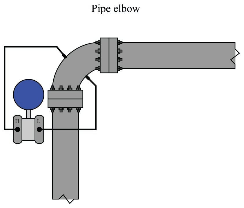
Pipe elbows should be considered for flow measurement only as a last resort. Their inaccuracies tend to be extreme, owing to the non-precise construction of most pipe elbows and the relatively weak differential pressures generated.
A final point should be mentioned on the subject of differential-producing elements, and that is their energy dissipation. Orifice plates are simple and relatively inexpensive to install, but their permanent pressure loss is high compared with other primary elements such as venturi tubes. Permanent pressure loss is permanent energy loss from the flowstream, which usually represents a loss in energy invested into the process by pumps, compressors, and/or blowers. Fluid energy dissipated by an orifice plate thus (usually) translates into a requirement of greater energy input to that process.
With the financial and ecological costs of energy being non-trivial in our modern world, it is important to consider energy loss as a significant factor in choosing the appropriate primary element for a pressure-based flowmeter. It might very well be that an “expensive” venturi tube saves more money in the long term than a “cheap” orifice plate, while delivering greater measurement accuracy as an added benefit.
Proper installation
Perhaps the most common way in which the flow measurement accuracy of any flowmeter becomes compromised is incorrect installation, and pressure-based flowmeters are no exception to this rule. The following list shows some of the details one must consider in installing a pressure-based flowmeter element:
- Necessary upstream and downstream straight-pipe lengths
- Beta ratio (ratio of orifice bore diameter to pipe diameter: \(\beta = {d \over D}\))
- Impulse tube tap locations
- Tap finish
- Transmitter location in relation to the pipe
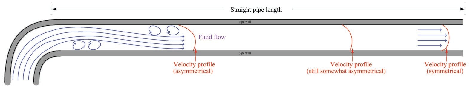
Sharp turns in piping networks introduce large-scale turbulence into the flowstream. Elbows, tees, valves, fans, and pumps are some of the most common causes of large-scale turbulence in piping systems. Successive pipe elbows in different planes are some of the worst offenders in this regard. When the natural flow path of a fluid is disturbed by such piping arrangements, the velocity profile of that fluid becomes distorted; e.g. the velocity gradient from one wall boundary of the pipe to the other will not be orderly. Large eddies in the flowstream (called swirl) will appear. This may cause problems for pressure-based flow elements which rely on linear acceleration (change in velocity in one dimension) to measure fluid flow rate. If the flow profile is distorted enough, the acceleration detected at the element may be too great or too little, and therefore not properly represent the full fluid flowstream. For this reason, pressure-based flowmeters should always be located upstream of major disturbances such as control valves and pipe elbows where possible.
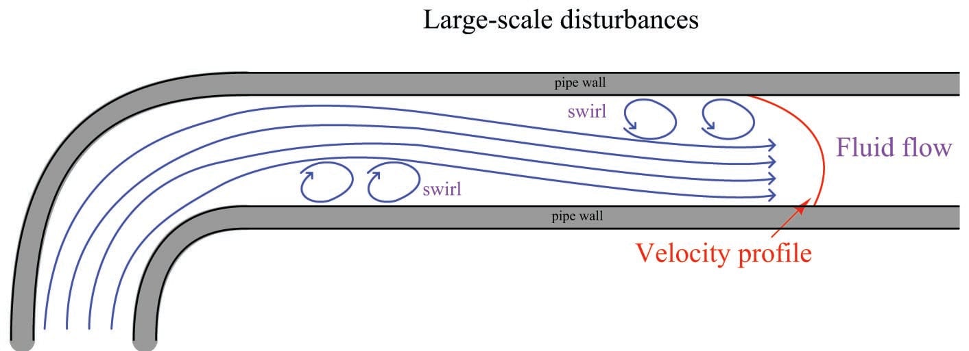
Even disturbances located downstream of the flow element may affect measurement accuracy if the disturbances are severe enough and/or close enough to the flow element. Unfortunately, both upstream and downstream flow disturbances are unavoidable on all but the simplest fluid systems. This means we must devise ways to stabilize a flowstream’s velocity profile near the flow element in order to achieve accurate measurements of flow rate. A very simple and effective way to stabilize a flow profile is to provide adequate lengths of straight pipe ahead of (and behind) the flow element. Given enough time, even the most chaotic flowstream will “settle down” to a symmetrical profile all on its own. The following illustration shows the effect of a pipe elbow on a flowstream, and how the velocity profile returns to a normal (symmetrical) form after traveling through a sufficient length of straight pipe:
Recommendations for minimum upstream and downstream straight-pipe lengths vary significantly with the nature of the turbulent disturbance, piping geometry, and flow element. As a general rule, elements having a smaller beta ratio (ratio of throat diameter \(d\) to pipe diameter \(D\)) are more tolerant of disturbances, with profiled flow devices (e.g. venturi tubes, flow tubes, V-cones) having the greatest tolerance. Ultimately, you should consult the flow element manufacturer’s documentation for a more detailed recommendation appropriate to any specific application.
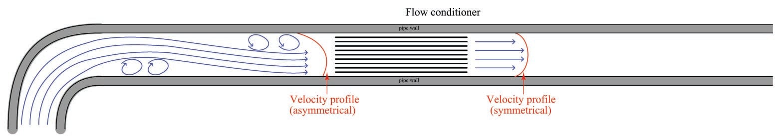
In applications where sufficient straight-run pipe lengths are impractical, another option exists for “taming” turbulence generated by piping disturbances. Devices called flow conditioners may be installed upstream of the flow element to help the flow profile achieve symmetry in a far shorter distance than simple straight pipe could do alone. Flow conditioners take the form of a series of tubes or vanes installed inside the pipe, parallel to the direction of flow. These tubes or vanes force the fluid molecules to travel in straighter paths, thus stabilizing the flowstream prior to entering a flow element:
This next photograph shows a very poor orifice plate installation, where the straight-run pipe requirements were completely ignored:
Not only is the orifice plate placed much too close to an elbow, the elbow happens to be on the upstream side of the orifice plate, where disturbances have the greatest effect! The saving grace of this installation is that it is not used for critical monitoring or control: it is simply a manual indication of air flow rate where accuracy is not terribly important. Nevertheless, it is sad to see how an orifice meter installation could have been so easily improved with just a simple re-location of the orifice plate along the piping length.
Poor installations such as this are surprisingly common, owing to the ignorance many piping designers have of flowmeter design and operating principles. Of all the criteria which must be balanced when designing a piping layout, optimum flowmeter location is often placed low in the order of importance (if it appears at all!). In applications where accuracy is important, flowmeter location needs to be a very high priority even if it means a more expensive, cumbersome, and/or unattractive piping design.
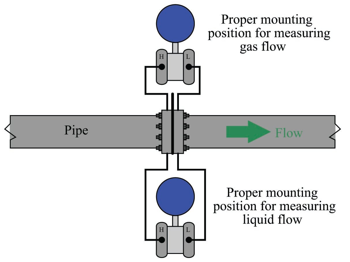
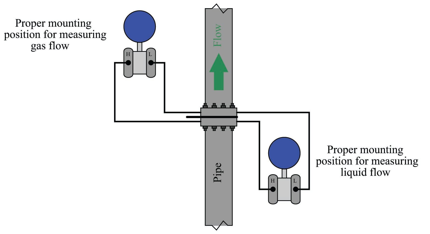
Another common source of trouble for pressure-based flowmeters is improper transmitter location. Here, the type of process fluid flow being measured dictates how the pressure-sensing instrument should be located in relation to the pipe. For gas and vapor flows, it is important that no stray liquid droplets collect in the impulse lines leading to the transmitter, lest a vertical liquid column begin to collect in those lines and generate an error-producing pressure. For liquid flows, it is important that no gas bubbles collect in the impulse lines, or else those bubbles may displace liquid from the lines and thereby cause unequal vertical liquid columns, which would (again) generate an error-producing differential pressure.
In order to let gravity do the work of preventing these problems, we must locate the transmitter above the pipe for gas flow applications and below the pipe for liquid flow applications. This illustration shows both installations for a horizontal pipe:
This next illustration shows both installations on a vertical pipe:
Condensible vapor applications (such as steam flow measurement) have traditionally been treated similarly to liquid measurement applications. Here, condensed liquid will collect in the transmitter’s impulse lines so long as the impulse lines are cooler than the vapor flowing through the pipe (which is typically the case). Placing the transmitter below the pipe allows vapors to condense and fill the impulse lines with liquid (condensate), which then acts as a natural seal protecting the transmitter from exposure to hot process vapors.
In such applications it is important for the technician to pre-fill both impulse lines with condensed liquid prior to placing the flowmeter into service. “Tee” fittings with removable plugs or fill valves are provided to do this. Failure to pre-fill the impulse lines will likely result in measurement errors during initial operation, as condensed vapors will inevitably fill the impulse lines at slightly different rates and cause a difference in vertical liquid column heights within those lines.
It should be noted that some steam flow element installations, however, will work well if the impulse lines are above the pipe. If such an installation is possible, the advantage of not having to deal with pre-filling impulse lines (or waiting for steam to condense to equal levels in both lines) are significant. For more information, I recommend consulting the Rosemount whitepaper entitled “Top Mount Installation for DP Flowmeters in Steam Service” (document 00870-0200-4809 first published August 2009).
If tap holes must be drilled into the pipe (or flanges) at the process site, great care must be taken to properly drill and de-burr the holes. A pressure-sensing tap hole should be flush with the inner pipe wall, with no rough edges or burrs to create turbulence. Also, there should be no reliefs or countersinking near the hole on the inside of the pipe. Even small irregularities at the tap holes may generate surprisingly large flow-measurement errors.
High-accuracy flow measurement
When we derived a formula for predicting flow rate from pressure dropped by a venturi tube (or orifice), we had to make many assumptions, chief among them being a total lack of friction (i.e. no energy dissipated due to friction) within the moving fluid and perfect stream-line flow (i.e. complete lack of turbulence). Suffice it to say, the flow formulae you have seen so far in this chapter are only approximations of reality. Orifice plates are some of the worst offenders in this regard, since the fluid encounters such abrupt changes in geometry passing through the orifice. Venturi tubes are nearly ideal, since the machined contours of the tube ensure gradual changes in fluid pressure and minimize turbulence.
However, in the real world we must often do the best we can with imperfect technologies. Orifice plates, despite being less than perfect as flow-sensing elements, are convenient and economical to install in flanged pipes. Orifice plates are also the easiest type of flow element to replace in the event of damage or routine servicing. In applications such as custody transfer (also called “fiscal” measurement), where the flow of fluid represents product being bought and sold, flow measurement accuracy is paramount. It is therefore important to figure out how to coax the most accuracy from the common orifice plate in order that we may measure fluid flows both accurately and economically.
If we compare the true flow rate through a pressure-generating primary sensing element against the theoretical flow rate predicted by an idealized equation, we may notice a substantial discrepancy. Causes of this discrepancy include, but are not limited to:
- Energy losses due to turbulence and viscosity
- Energy losses due to friction against the pipe and element surfaces
- Unstable location of vena contracta with changes in flow
- Uneven velocity profiles caused by irregularities in the pipe
- Fluid compressibility
- Thermal expansion (or contraction) of the element and piping
- Non-ideal pressure tap location(s)
- Excessive turbulence caused by rough internal pipe surfaces
The ratio between true flow rate and theoretical flow rate for any measured amount of differential pressure is known as the discharge coefficient of the flow-sensing element, symbolized by the variable \(C\). Since a value of 1 represents a theoretical ideal, the actual value of \(C\) for any real pressure-generating flow element will be less than 1:
\[C = {\hbox{True flow} \over \hbox{Theoretical flow}}\]
For gas and vapor flows, true flow rate deviates even more from the theoretical (ideal) flow value than liquids do, for reasons that have to do with the compressible nature of gases and vapors. A gas expansion factor (\(Y\)) may be calculated for any flow element by comparing its discharge coefficient for gases against its discharge coefficient for liquids. As with the discharge coefficient, values of \(Y\) for any real pressure-generating element will be less than 1:
\[Y = {C_{gas} \over C_{liquid}}\]
\[Y = {\left({\hbox{True gas flow} \over \hbox{Theoretical gas flow}}\right) \over \left({\hbox{True liquid flow} \over \hbox{Theoretical liquid flow}}\right)}\]
Incorporating these factors into the ideal volumetric flow equation developed on in section [Ideal flow equation], we arrive at the following formulation:
\[Q = \sqrt{2} {C Y A_2 \over \sqrt{1 - \left({A_2 \over A_1}\right)^2}} \sqrt{{P_1 - P_2} \over \rho}\]
If we wished, we could even add another factor to account for any necessary unit conversions (\(N\)), getting rid of the constant \(\sqrt{2}\) in the process:
\[Q = N {C Y A_2 \over \sqrt{1 - \left({A_2 \over A_1}\right)^2}} \sqrt{{P_1 - P_2} \over \rho}\]
Sadly, neither the discharge coefficient (\(C\)) nor the gas expansion factor (\(Y\)) will remain constant across the entire measurement range of any given flow element. These variables are subject to some change with flow rate, which further complicates the task of accurately inferring flow rate from differential pressure measurement. However, if we know the values of \(C\) and \(Y\) for typical flow conditions, we may achieve good accuracy most of the time.
Likewise, the fact that \(C\) and \(Y\) change with flow places limits on the accuracy obtainable with the “proportionality constant” formulae seen earlier. Whether we are measuring volumetric or mass flow rate, the \(k\) factor calculated at one particular flow condition will not hold constant for all flow conditions:
\[Q = k \sqrt{{P_1 - P_2} \over \rho}\]
\[W = k \sqrt{\rho(P_1 - P_2)}\]
This means after we have calculated a value for \(k\) based on a particular flow condition, we can only trust the results of the equation for flow conditions not too different from the one we used to calculate \(k\).
As you can see in both flow equations, the density of the fluid (\(\rho\)) is an important factor. If fluid density is relatively stable, we may treat \(\rho\) as a constant, incorporating its value into the proportionality factor (\(k\)) to make the two formulae even simpler:
\[Q = k_Q \sqrt{P_1 - P_2}\]
\[W = k_W \sqrt{P_1 - P_2}\]
However, if fluid density is subject to change over time, we will need some means to continually calculate \(\rho\) so our inferred flow measurement will remain accurate. Variable fluid density is a typical state of affairs in gas flow measurement, since all gases are compressible by definition. A simple change in static gas pressure within the pipe is all that is needed to make \(\rho\) change, which in turn affects the relationship between flow rate and differential pressure drop.
The American Gas Association (AGA) provides a formula for calculating volumetric flow of any gas using orifice plates in their #3 Report, compensating for changes in gas pressure and temperature. A variation of that formula is shown here (consistent with previous formulae in this section):
\[Q = N {{C Y A_2} \over \sqrt{1 - \left({A_2 \over A_1}\right)^2}} \sqrt{{Z_s P_1 (P_1 - P_2)} \over {G_f Z_{f1} T}}\]
Where,
\(Q\) = Volumetric flow rate (SCFM = standard cubic feet per minute)
\(N\) = Unit conversion factor
\(C\) = Discharge coefficient (accounts for energy losses, Reynolds number corrections, pressure tap locations, etc.)
\(Y\) = Gas expansion factor
\(A_1\) = Cross-sectional area of mouth
\(A_2\) = Cross-sectional area of throat
\(Z_s\) = Compressibility factor of gas under standard conditions
\(Z_{f1}\) = Compressibility factor of gas under flowing conditions, upstream
\(G_f\) = Specific gravity of gas (density compared to ambient air)
\(T\) = Absolute temperature of gas
\(P_1\) = Upstream pressure (absolute)
\(P_2\) = Downstream pressure (absolute)
This equation implies the continuous measurement of absolute gas pressure (\(P_1\)) and absolute gas temperature (\(T\)) inside the pipe, in addition to the differential pressure produced by the orifice plate (\(P_1 - P_2\)). These measurements may be taken by three separate devices, their signals routed to a gas flow computer:
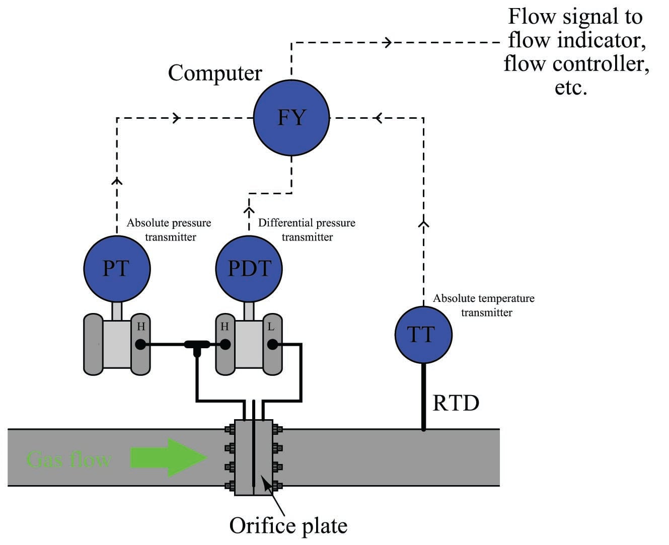
Note the location of the RTD (thermowell), positioned downstream of the orifice plate so the turbulence it generates will not create additional turbulence at the orifice plate. The American Gas Association (AGA) allows for upstream placement of the thermowell, but only if located at least three feet upstream of a flow conditioner.
In order to best control all the physical parameters necessary for good orifice metering accuracy, it is standard practice for custody transfer flowmeter installations to use honed meter runs rather than standard pipe and pipe fittings. A “honed run” is a complete piping assembly consisting of a manufactured fitting to hold the orifice plate and sufficient straight lengths of pipe upstream and downstream, the interior surfaces of that pipe machined (“honed”) to have a glass-smooth surface with precise and symmetrical dimensions. Honed runs ensure minimum disruption to the flowing gas or liquid, thus improving measurement accuracy by avoiding unnecessary turbulence and/or distorted flow profiles. Such piping “runs” are quite expensive, but necessary to achieve flow measurement accuracy worthy of custody transfer.
This photograph shows a set of AGA3-compliant orifice meter runs measuring the flow of natural gas:
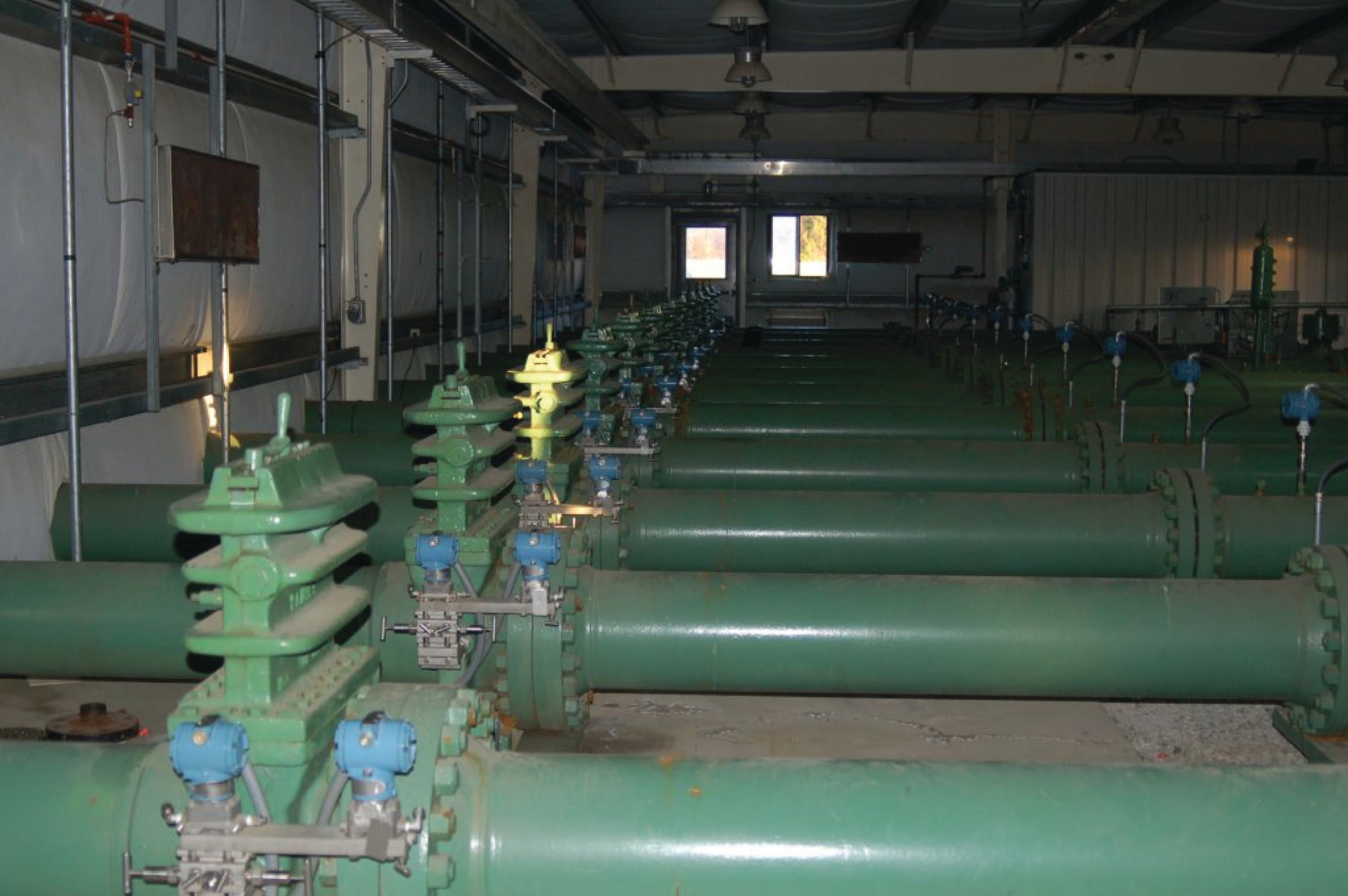
Note the special transmitter manifolds, built to accept both the differential pressure and absolute pressure (Rosemount model 3051) transmitters. Also note the quick-change fittings (the ribbed metal housings) holding the orifice plates, to facilitate convenient change-out of the orifice plates which is periodically necessary due to wear. It is not unheard of to replace orifice plates on a daily basis in some industries to ensure the sharp orifice edges necessary for accurate measurement.
Although not visible in this photograph, these meter runs are connected together by a network of shut-off valves directing the flow of natural gas through as few meter runs as desired. When the total gas flow rate is great, all meter runs are placed into service and their respective flow rates summed to yield a total flow measurement. When the total flow rate decreases, individual meter runs are shut off, resulting in increased flow rates through the remaining meter runs. This “staging” of meter runs expands the effective turndown or rangeability of the orifice plate as a flow-sensing element, resulting in much more accurate flow measurement over a wide range of flow rates than if a single (large) orifice meter run were used.
An alternative to multiple instruments (differential pressure, absolute pressure, and temperature) installed on each meter run is to use a single multi-variable transmitter capable of measuring gas temperature as well as both static and differential pressures. This approach enjoys the advantage of simpler installation over the multi-instrument approach:
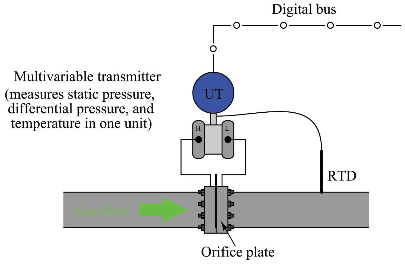
The Rosemount model 3095MV and Yokogawa model EJX910 are examples of multi-variable transmitters designed to perform compensated gas flow measurement, equipped with multiple pressure sensors, a connection port for an RTD temperature sensor, and sufficient digital computing power to continuously calculate flow rate based on the AGA equation. Such multi-variable transmitters may provide an analog output for computed flow rate, or a digital output where all three primary variables and the computed flow rate may be transmitted to a host system (as shown in the previous illustration). The Yokogawa EJX910A provides an interesting signal output option: a digital pulse signal, where each pulse represents a specific quantity (either volume or mass) of fluid. The frequency of this pulse train represents flow rate, while the total number of pulses counted over a period of time represents the total amount of fluid that has passed through the orifice plate over that amount of time.
This photograph shows a Rosemount 3095MV transmitter used to measure mass flow on a pure oxygen (gas) line. The orifice plate is an “integral” unit immediately below the transmitter body, sandwiched between two flange plates on the copper line. A three-valve manifold interfaces the model 3095MV transmitter to the integral orifice plate structure:
The temperature-compensation RTD may be clearly seen on the left-hand side of the photograph, installed at the elbow fitting in the copper pipe.
Liquid flow measurement applications may also benefit from compensation, because liquid density changes with temperature. Static pressure is not a concern here, because liquids are considered incompressible for all practical purposes. Thus, the formula for compensated liquid flow measurement does not include any terms for static pressure, just differential pressure and temperature:
\[Q = N {{C Y A_2} \over \sqrt{1 - \left({A_2 \over A_1}\right)^2}} \sqrt{{(P_1 - P_2)[1 + k_T(T - T_{ref})]}}\]
The constant \(k_T\) shown in the above equation is the proportionality factor for liquid expansion with increasing temperature. The difference in temperature between the measured condition (\(T\)) and the reference condition (\(T_{ref}\)) multiplied by this factor determines how much less dense the liquid is compared to its density at the reference temperature. It should be noted that some liquids – notably hydrocarbons – have thermal expansion factors significantly greater than water. This makes temperature compensation for hydrocarbon liquid flow measurement very important if the measurement principle is volumetric rather than mass-based.
Equation summary
Volumetric flow rate (\(Q\)) full equation:
\[Q = N {{C Y A_2} \over \sqrt{1 - \left({A_2 \over A_1}\right)^2}} \sqrt{{P_1 - P_2} \over \rho_f}\]
Volumetric flow rate (\(Q\)) simplified equation:
\[Q = k \sqrt{{P_1 - P_2} \over \rho_f}\]
Mass flow rate (\(W\)):
\[W = N {{C Y A_2} \over \sqrt{1 - \left({A_2 \over A_1}\right)^2}} \sqrt{\rho_f (P_1 - P_2)}\]
Mass flow rate (\(W\)) simplified equation:
\[W = k \sqrt{\rho_f (P_1 - P_2)}\]
Where,
\(Q\) = Volumetric flow rate (e.g. gallons per minute, flowing cubic feet per second)
\(W\) = Mass flow rate (e.g. kilograms per second, slugs per minute)
\(N\) = Unit conversion factor
\(C\) = Discharge coefficient (accounts for energy losses, Reynolds number corrections, pressure tap locations, etc.)
\(Y\) = Gas expansion factor (\(Y = 1\) for liquids)
\(A_1\) = Cross-sectional area of mouth
\(A_2\) = Cross-sectional area of throat
\(\rho_f\) = Fluid density at flowing conditions (actual temperature and pressure at the element)
\(k\) = Constant of proportionality (determined by experimental measurements of flow rate, pressure, and density)
The beta ratio (\(\beta\)) of a differential-producing element is the ratio of throat diameter to mouth diameter (\(\beta = {d \over D}\)). This is the primary factor determining acceleration as the fluid increases velocity entering the constricted throat of a flow element (venturi tube, orifice plate, wedge, etc.). The following expression is often called the velocity of approach factor (commonly symbolized as \(E_v\)), because it relates the velocity of the fluid through the constriction to the velocity of the fluid as it approaches the flow element:
\[E_v = {1 \over \sqrt{1 - \beta^4}} = \hbox{ Velocity of approach factor}\]
This same velocity approach factor may be expressed in terms of mouth and throat areas (\(A_1\) and \(A_2\), respectively):
\[E_v = {1 \over \sqrt{1 - \left(A_2 \over A_1\right)^2}} = \hbox{ Velocity of approach factor}\]
Beta ratio has a significant impact on the number of straight-run pipe lengths needed to condition the flow profile upstream and downstream of the flow element. Large beta ratios (where the bore diameter approaches the flowtube’s inside diameter) are more sensitive to piping disturbances, since there is less acceleration of the flowstream through the element, and therefore flow profile asymmetries caused by piping disturbances are significant in comparison to the fluid’s through-bore velocity. Small beta ratio values correspond to larger acceleration factors, where disturbances in the flow profile become “swamped” by the high throat velocities created by the element’s constriction. A disadvantage of small beta ratio values is that the flow element exhibits a greater permanent pressure loss, which is an operational cost if the flow is provided by a machine such as an engine- or motor-driven pump (more energy required to turn the pump, equating to a greater operating cost to run the process).
When computing the volumetric flow of a gas in standard volume units (e.g. SCFM), the equation becomes much more complex than the simple (flowing) volumetric rate equation. Any equation computing flow in standard units must predict the effective expansion of the gas if it were to transition from flowing conditions (the actual pressure and temperature it experiences flowing through the pipe) to standard conditions (one atmosphere pressure at 60 degrees Fahrenheit). The compensated gas flow measurement equation published by the American Gas Association (AGA Report #3) in 1992 for orifice plates with flange taps calculates this expansion to standard conditions with a series of factors accounting for flowing and standard (“base”) conditions, in addition to the more common factors such as velocity of approach and gas expansion. Most of these factors are represented in the AGA3 equation by different variables beginning with the letter \(F\):
\[Q = F_n (F_c + F_{sl}) Y F_{pb} F_{tb} F_{tf} F_{gr} F_{pv} \sqrt{h_W P_{f1}}\]
Where,
\(Q\) = Volumetric flow rate (standard cubic feet per hour – SCFH)
\(F_n\) = Numeric conversion factor (accounts for certain numeric constants, unit-conversion coefficients, and the velocity of approach factor \(E_v\))
\(F_c\) = Orifice calculation factor (a polynomial function of the orifice plate’s \(\beta\) ratio and Reynolds number), appropriate for flange taps
\(F_{sl}\) = Slope factor (another polynomial function of the orifice plate’s \(\beta\) ratio and Reynolds number), appropriate for flange taps
\(F_c + F_{sl}\) = \(C_d\) = Discharge coefficient, appropriate for flange taps
\(Y\) = Gas expansion factor (a function of \(\beta\), differential pressure, static pressure, and specific heats)
\(F_{pb}\) = Base pressure factor = \({14.73 \hbox{ PSI} \over P_b}\), with pressure in PSIA (absolute)
\(F_{tb}\) = Base temperature factor = \({T_b \over 519.67}\), with temperature in degrees Rankine
\(F_{tf}\) = Flowing temperature factor = \(\sqrt{519.67 \over T_f}\), with temperature in degrees Rankine
\(F_{gr}\) = Real gas relative density factor = \(\sqrt{1 \over G_r}\)
\(F_{pv}\) = Supercompressibility factor = \(\sqrt{Z_b \over Z_{f1}}\)
\(h_W\) = Differential pressure produced by orifice plate (inches water column)
\(P_{f1}\) = Flowing pressure of gas at the upstream tap (PSI absolute)
