Facebook
 Google
 GitHub
 Linkedin
System Dynamic and Frequency Response Analysis
Understanding the building blocks of s-domain analysis and magnitude response theory can go a long way in helping engineers predict how and why some system design choices are made over others.
Previously, Control.com published two articles about system dynamic response and the transfer function, covering some basics of control theory along the way. The first article, Introduction to System Dynamic Responses, introduced how the study of system dynamics can help engineers better understand the relationships between a complex system’s inputs and outputs. In the second article, Introduction to Transfer Functions for Control System Analysis, we dove deeper into the equations that define these input and output relationships. These first two articles introduced the concepts of the Laplace transform and the frequency domain, which are mathematical tools that can help us solve complex equations in control theory relatively simply.

Figure 1. An abstract representation of various signals at different frequencies. Image used courtesy of Adobe Stock
In this third article, we examine frequency response further, starting with more basic definitions followed by case examples covering some real-life scenarios. Like the previous articles in the series, it’s not intended to be a classroom lesson in control theory – rather a more holistic treatment of the fundamentals behind these complex engineering equations.
What is Frequency Response Analysis?
As we learned previously, we employ the transfer function in control engineering to convert complex differential equations in the time domain into more simple algebraic expressions in the frequency domain, also known as the s-domain. S-domain formulas offer an efficient way to evaluate how our system would respond to different inputs. Because we are doing this in the frequency domain, the evaluation method has been dubbed frequency response.

Figure 2. Sound wave analysis is one common application of frequency response. Image used courtesy of Adobe Stock
Many physical phenomena are easier to interpret and manipulate in the frequency domain. For instance, sound can be represented as s-domain sinusoidal waves of which changes in frequency and amplitude help us understand things like distortion and amplification. There are also mathematical operations that can be hard to execute in the time domain rather than in the s-domain. For example, signal convolution becomes an algebraic multiplication in the frequency domain.
Bode Plots for Frequency Analysis
To make frequency response easier to interpret and visualize, we make use of Bode plots. Bode plots consist of two graphs, one of which is used to illustrate the gain response and the other one for the phase response, both expressed in terms of frequency. Let us remember that gain (or magnitude) and phase are the two parameters essential to defining a frequency-domain plot.
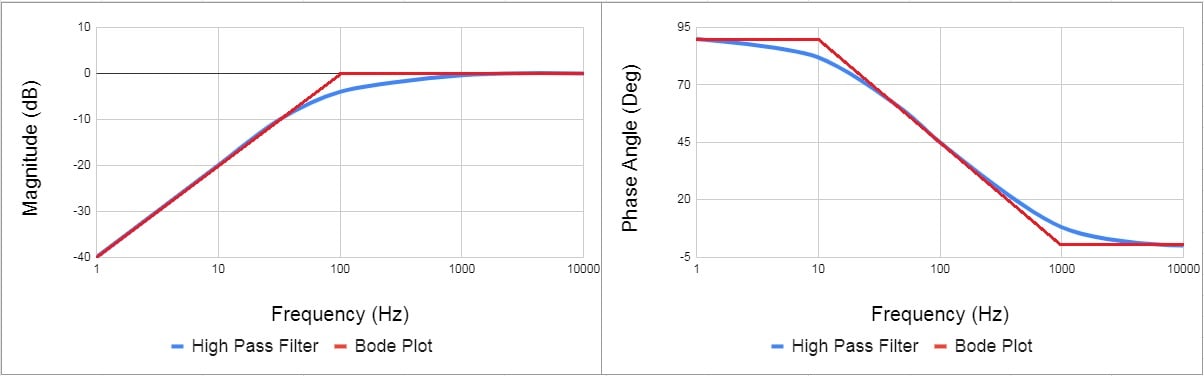
Figure 3. A Bode plot consists of two graphs, one for magnitude and the other for phase changes.
The gain or magnitude is plotted along the first graph's vertical axis and measured in Decibels (dB), a logarithmic scale. The second graph illustrates the phase which is commonly expressed in degrees or radians. Both of these axis definitions are described in greater depth below.
Magnitude Response
Magnitude response aims to understand how changes in the input affect the strength of our system’s output. Output signals can be amplified, or they can be attenuated. We can also manipulate the inputs to produce desired magnitude changes at specific frequencies. This is one of the tools available in control systems to customize and optimize different real-world applications.
Perhaps the first physical phenomenon that comes to mind is sound followed by the multitude of devices and applications available in the industry to manipulate it. For example, sound amplifiers use magnitude response techniques to strengthen sound, doing so at specific frequency ranges when needed. This helps isolate and improve sound waves coming from different instruments and sources.
Magnitude response analysis is also crucial in communication systems, especially wireless systems. Conducting an s-domain analysis can be a very helpful way to identify and solve issues with interference and attenuation.
Applications of magnitude response can also be found in the healthcare industry. For example, magnetic resonance imaging (MRI) and ultrasound diagnostic imaging devices both use magnitude filters to improve the quality of the image, which contributes to more accurate diagnoses and better patient outcomes.

Figure 4. MRI scans rely on a careful calibration of magnitude and phase to produce high-quality diagnostic and patient results. Image used courtesy of Adobe Stock
Phase Response
A change or offset in the frequency domain is equivalent to a delay in the time domain. Therefore, the goal of the phase response analysis is to understand when these delays occur upon changes in the input, as well as to maintain synchronicity in some systems.
In many industries, signal equalization is essential for maintaining quality and fidelity. Calibrating the phase response helps keep long-distance communication free of distortion and interference. Generally, any control system requires a proper tuning of frequency phases to ensure stability.
Phase and magnitude changes are the key characteristics that help us quantify how our system’s output is affected by changes in the input. Now, let’s review some of the different forms of input waves used in these analyses.
Inputs
Below are some simple waveforms commonly used as inputs in system dynamic response. These common scenarios represent most real-world inputs, both from natural forces and external control devices.
Impulse
An impulse is an instantaneous spike. It is plotted as having virtually infinite amplitude and nearly zero duration. This waveform aims to represent what occurs in the real world when there are sudden increases of energy at the input that are orders of magnitude more than the typical working range. Think about an electrical current spike on the initial startup of a motor or a capacitive device.
Step Input
The step signal indicates a sudden change in the input that remains constant at a certain value for some time. The goal of the analysis is to understand the response of the output when the input then remains constant. Think of a signal to an actuator or proportional valve commanding a set position until a new command is issued.
Ramp Input
This is a straight line that represents a linear increase or decrease at the input. Soft starts and VFDs are commonly found providing a ramped input to a motion system.
Sinusoidal
The most basic form that provides a comprehensive frequency response analysis. The amplitude and frequency of the wave may be changed throughout the test to see the effects in the output. Electrical, audio, and many mechanical cycles provide this sinusoidal input.
Complex Signals
There are several more complex signals able to be employed here. In any case, the Bode plot helps represent and evaluate the outputs.
Frequency Response Analysis Summary
Analyzing a system to predict such behavior is useful for most motion, electrical, and audio systems, among others. Familiarity with the methods and theories used in this analysis is often outside the scope of many engineers and technicians. However, understanding the building blocks of these theories can go a long way to help predict how and why some system design choices are made over others.