Facebook
 Google
 GitHub
 Linkedin
Introduction to Transfer Functions for Control System Analysis
Transfer functions allow systems to be converted from non-algebraic time measurement units into equations that can be solved, but how do these functions work, and why do we use them?
In the previous article, we talked about the basics of system dynamics. We also covered the concept of complexity as it relates to control theory. In a complex electromechanical system, there can be many elements and rules and a certain degree of uncertainty about the output. To understand such systems, the output and other unknowns of the system must be evaluated upon different inputs. This process is the basis for system dynamics response.
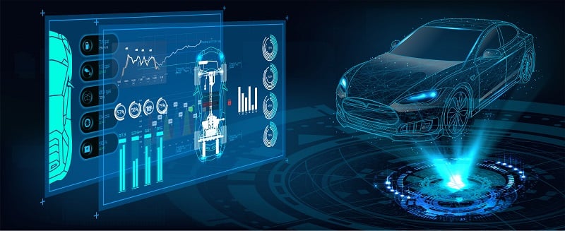
Figure 1. Cars are good examples of complex electrical and mechanical control systems. Image used courtesy of Adobe Stock
In this article, we will dive deeper into the mathematical relationships between the elements of mechanical and electrical control systems. We will then learn about the transfer function.
What is the transfer function and why do we use it? You have likely already found numerous websites, articles, and white papers covering this topic. Our goal with this article is to help understand the reasoning behind the concepts rather than a textbook class in control theory.
Differential Equations in Electronics
Let us begin with understanding the relationships between the different elements of a control system. As we know, voltage and current are the basis for any electrical circuit. Also, the common tangible electrical circuit elements include resistors, capacitors, and inductors. We also know that voltage represents a potential difference between two points and that current is the rate of change in the motion of electrons.
Important elements of a mechanical circuit include mass, springs, and resistances. The relationships between these elements establish motion, velocity, and acceleration equations. The rate of change of position of a body or mass is the velocity. Similarly, the rate of change of the velocity is the acceleration.
Rates of change are also known as derivatives. Mathematically, rates of change are represented as differential functions or equations.
To exemplify this, let us use a simple loop RLC electrical circuit. Such a circuit consists of a resistor, an inductor, and a capacitor connected in series to a power source.
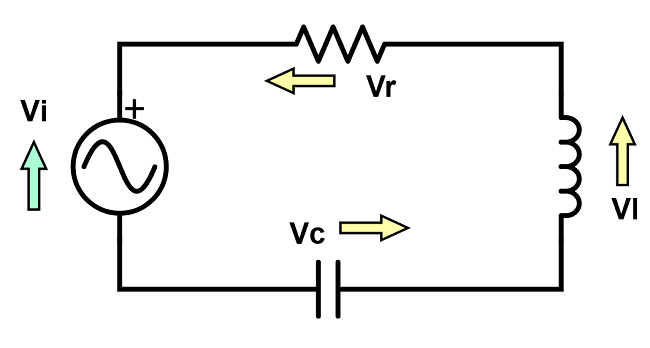
Figure 2. A simple series RLC series circuit.
According to Kirchhoff’s voltage law, the sum of voltages within a closed loop is always zero. This circuit contains a single power supply (Vi) and three power-consuming elements: the resistor (VR), the inductance (VL), and the capacitance (VC). Considering this, the equation for this circuit would be as follows:
$$V_i-V_R-V_L-V_C=0$$
$$V_i=V_R+V_L+V_C$$
Voltage of Resistors
Now, let us analyze each element separately. We know the function of resistors is to reduce current flow. Ohm’s Law establishes a relationship between the voltage across a resistor and the current passing through it. The proportionality is established by the resistance value (R).
$$V_R(t)=R \cdot I(t)$$
The equation is expressed as a function of time because the voltage at any given time is given by the contemporaneous current multiplied by the resistance factor. The following equations are also in the time domain.
Voltage of Inductors
Inductors are used for filtering out noise and signal conditioning. They are also called coils or chokes. As current flows through the coil in an inductor, a magnetic field is induced into a conductor, temporarily storing the energy to release it back to the circuit. The voltage-current relationship for an inductor is shown in the equation below. L is the inductance coefficient of the component, measured in Henries.
$$V_L(t)=L \cdot {dI(t) \over dt}$$
Voltage of Capacitors
Finally, we have the capacitor. These devices can store electrical energy using special arrays of metallic plates and dielectric media. Mathematically, capacitors are inverse to inductors. Capacitance is measured in Farads.
$$I(t)=C \cdot {dV(t) \over dt}$$
To express this as a voltage function, we solve for V(t).
$$V_C(t)={1 \over C} \int_{0}^{t} I(t) \,dt$$
Let’s substitute all three voltage expressions into our original circuit equation.
$$V_i(t)=V_R(t)+V_L(t)+V_C(t)$$
$$V_i(t)=RI(t)+{dI(t) \over dt}+\int_{0}^{t} I(t) \,dt$$
We have differentials and integrals in the resulting equation. To simplify it, we will differentiate both sides, resulting in the following:
$$V_i(t)=R{dI(t) \over dt}+L{dI^2(t) \over dt^2}+{1 \over C}I(t)$$
$$L{dI^2(t) \over dt^2}+R{dI(t) \over dt}+{1 \over C}I(t)=0$$
What we have as a result is a second order differential equation that represents the RLC circuit. Now, let us pause for a moment and reflect on how a very simple electrical circuit with only three elements led to this equation. Can you imagine what sort of equations are needed to represent more complex systems found in real life?
To solve such systems more efficiently, we can use the transfer function, which is based on the Laplace transform.
The Laplace Transform
The Laplace transform was one of the greatest discoveries in mathematics. It is named after eighteenth-century French mathematician Pierre-Simon Laplace. The Laplace transform is a method that performs a transformation to a mathematical equation, as indicated by its name. Specifically, this transformation is done between the time and frequency domains.
Frequency Domain, or S-domain
Remember that our RLC circuit equation is in the time domain because voltage and current are expressed as time functions. If we apply the Laplace transform to this equation, we will move into the frequency domain. The frequency domain is also known as the s-domain. “s” is employed in the s-domain the same way that “t” is in the time domain.
But what is the whole purpose of the transformation? Simplification. You will see that complex differential equations have relatively simple algebraic function counterparts in the s-domain. In control engineering, it is commonplace to transform complex differential equations to the s-domain to solve them and then transform them back into the time domain. This last step is called Inverse Laplace Transform.

Figure 3. Mechanical systems that evaluate motion based on mass, damping, and spring forces must employ advanced analytical methods like the Laplace Transform. Image used courtesy of Adobe Stock
Now, what exactly is the Laplace transform? There are large amounts of literature out there covering all the mathematic calculations, as well as all the Laplace tables. We want to touch on the answer to the question: what exactly is it?
Everything starts with this formula:
$$L(f(t))=F(s)=\int_{0}^{-\infty} e^{-st}f(t) \,dt$$
The Laplace transform of a function of time results in a function of “s”, F(s). To calculate it, we multiply the function of time by \(e^{-st}\), and then integrate it. The resulting integral is then evaluated from zero to infinity. For this to be valid, the limits must converge.
Let’s summarize what the Laplace transform of the RLC circuit would look like. If you would like step-by-step walkthroughs on how to solve differential equations and Laplace transforms, we recommend the following site:
https://www.khanacademy.org/math/differential-equations
Starting with our original equation, we apply the Laplace transform:
$$L(V_i(t))=L(RI(t))+L\left(L {dI(t) \over dt}\right)+L\left({1 \over C}\int_{0}^{t} I(t) \,dt\right)$$
We use help from known Laplace transforms in Laplace tables and obtain the following. For simplicity, we will neglect the starting current I(0) at the inductor.
$${V \over s}=RI(s)+L\left(sI(s)-I(0)\right)+{I(s) \over sC}$$
$${V \over s}=RI(s)+LsI(s)+{I(s) \over sC}$$
Then, we continue to solve for I(s).
$${V \over s}=\left(R+sL+{1 \over sC}\right)I(s)$$
$$I(s)={V \over s(R+sL+{1 \over sC})}$$
Our final equation is:
$$I(s)={V \over s^2L+sR+{1 \over C}}$$
What we have is a relationship between voltage and current given by a simple quadratic polynomial. The solution is now algebraic, which is the greatest advantage of the Laplace transform applied in this context. This is also called the “Transfer Function”. Remember that the equation is in the s-domain, to return it to the time domain, you will need to do the Inverse Laplace transform.