 Facebook
 Google
 GitHub
 Linkedin
Ladder Diagram (LD) Structure Commands

How are function blocks, or structures, used in ladder logic programming?
In a PLC, structure commands combine the fundamental coils and contacts to form more complex operations of counting, timing, math, and even custom instructions. Without these advanced commands, many PLC operations would be impossible.
The simple PLC ladder diagram (LD) commands consist of contacts and coils, arranged in sequences that mimic industrial electrical control structures. However, a quick look at any PLC program will show advanced commands including counters, timers, comparison, mathematics, sequences, and even many user-defined structures that can greatly benefit the process. This section of the book will explain the most commonly found structure type commands.
PLC Counter Instructions
A counter is a PLC instruction that either increments (counts up) or decrements (counts down) an integer number value when prompted by the transition of a bit from 0 to 1 (“false” to “true”). Counter instructions come in three basic types: up counters, down counters, and up/down counters. Both “up” and “down” counter instructions have single inputs for triggering counts, whereas “up/down” counters have two trigger inputs: one to make the counter increment and one to make the counter decrement.
To illustrate the use of a counter instruction, we will analyze a PLC-based system designed to count objects as they pass down a conveyor belt:

In this system, a typical photoeye, or optoelectronic sensor beam causes the light sensor to close its output contact when an object is detected, energizing discrete channel In.1. When an object on the conveyor belt passes in front of the light beam from the source to the sensor, the sensor’s contact closes, passing power to input In.1. A pushbutton switch connected to activate discrete input In.0 when pressed will serve as a manual “reset” of the count value. An indicator lamp connected to one of the discrete output channels will serve as an indicator of when the object count value has exceeded some pre-set limit.
We will now analyze a simple Ladder Diagram program designed to increment a counter instruction each time the light beam breaks:
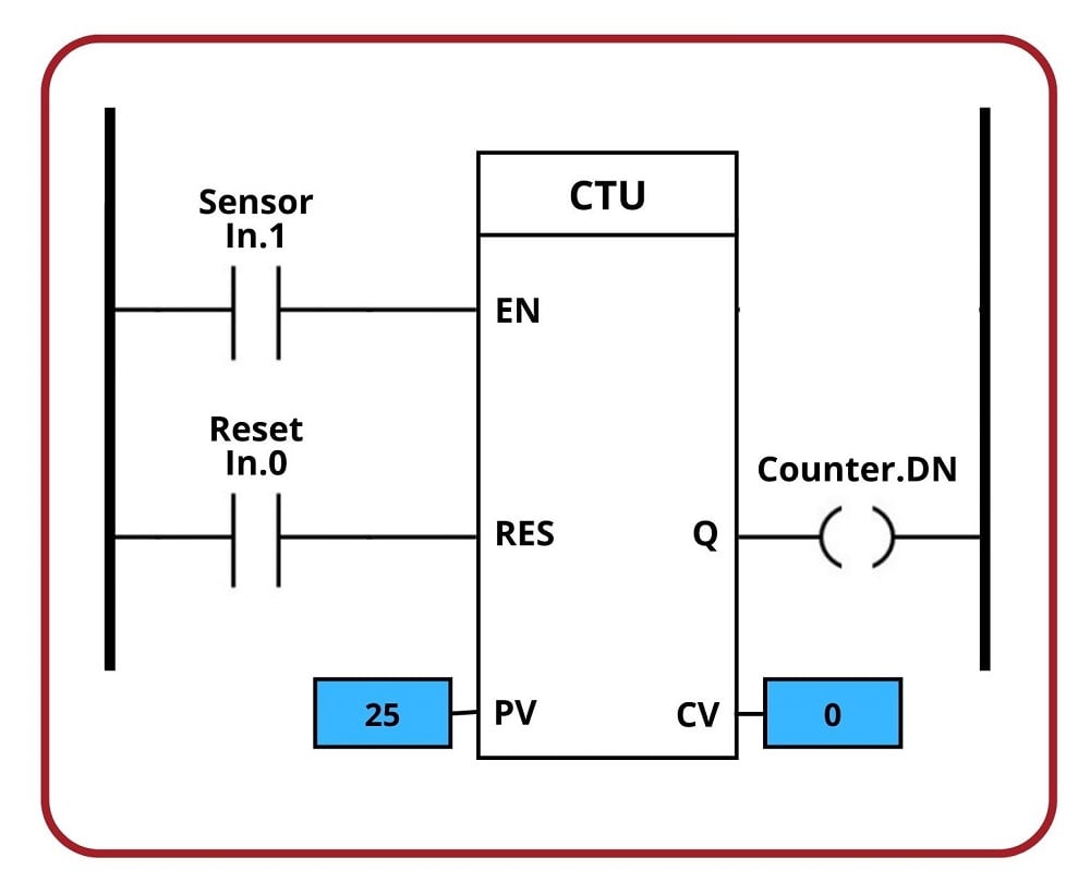
This particular counter instruction (CTU) is an incrementing counter, which means it counts “up” with each off-to-on transition input to its “EN” input. The normally-closed virtual contact (Sensor In.1) is typically held in the “open” state when the light beam is continuous, by virtue of the fact the sensor energizes the discrete input channel when the beam is broken by a passing object on the conveyor belt. When this happen, the input channel energizes, causing the virtual contact Sensor In.1 to “close” and send virtual power to the “EN” input of the counter instruction. This increments the counter just as the leading edge of the object breaks the beam. The second input of the counter instruction box (“RES”) is the reset input, receiving virtual power from the contact Reset In.0 whenever the reset pushbutton is pressed. If this input is activated, the counter immediately resets its current value (CV) to zero.
Status indication is shown in this Ladder Diagram program, with the counter’s preset value (PV) of 25 and the counter’s current value (CV) of 0 shown highlighted in blue. The preset value is something programmed into the counter instruction before the system is put into service, and it serves as a threshold for activating the counter’s output (Q), which in this case would be used to turn on the count indicator lamp (the Out.8 coil). According to the IEC 61131-3 programming standard, this counter output should activate whenever the current value is equal to or greater than the preset value (Q is active if CV \(\geq\) PV).
This is the status of the same program after more than 25 objects have passed by the sensor on the conveyor belt. As you can see, the current value of the counter has increased to 27, exceeding the preset value and activating the discrete output:

If we did not wish to count the number of events that have happened during a duration but instead wanted to track a current remaining value (like an inventory of parts being consumed by a process), we could use a down counter. Like with the up counter, the Q output is activated when the CV \(\geq\) PV, so it would be logical to use this output to track an inventory reaching a low stage. When the Q output turns off, it’s time to refill the part tray.

Up / Down Counters
A potential problem in either version of this object-counting system is that the PLC cannot discriminate between forward and reverse motion on the conveyor belt. If, for instance, the conveyor belt was ever reversed in direction, the sensor would continue to count objects that had already passed by before (in the forward direction) as those objects retreated on the belt. This would be a problem because the system would “think” more objects had passed along the belt (indicating greater production) than actually did.
One solution to this problem is to use an up/down counter, capable of both incrementing (counting up) and decrementing (counting down), and equip this counter with two light-beam sensors capable of determining the direction of travel. If two light beams are oriented parallel to each other, closer than the width of the narrowest object passing along the conveyor belt, we will have enough information to determine the direction of object travel:
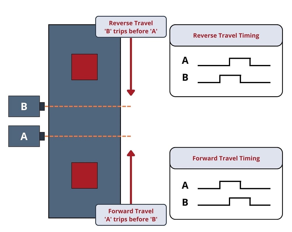
This is called quadrature signal timing, because the two pulse waveforms are approximately 90\(^{o}\) (one-quarter of a period) apart in phase. We can use these two phase-shifted signals to increment or decrement an up/down counter instruction, depending on which pulse leads and which pulse lags.
A Ladder Diagram PLC program designed to interpret the quadrature pulse signals is shown here, making use of negative-transition contacts as well as standard contacts:

The counter will increment (count up) when sensor B de-energizes only if sensor A is already in the de-energized state (i.e. light beam A breaks before B). The counter will decrement (count down) when sensor A de-energizes only if sensor B is already in the de-energized state (i.e. light beam B breaks before A).
The current value (CV) and the preset value (PV) of each counter is associated with a tag name of its own, in this case it might be Parts_Counted. The double integer (DINT) number of a counter’s current value (CV) is a variable in the PLC’s memory just like boolean values such as SensorA, SensorB, and Reset, and may be associated with a tag name or symbolic address just the same. This allows other instructions in a PLC program to read (and sometimes write!) values from and to that memory location.
PLC Timer Instructions
A timer is a PLC instruction measuring the amount of time elapsed following an event. Timer instructions come in two basic types: on-delay timers and off-delay timers. Both “on-delay” and “off-delay” timer instructions have single inputs triggering the timed function.
Most timers on modern PLCs have a time base that is either in milliseconds (where 1000 ms equals 1 second) or in selectable time bases of thousandths, hundredths, tenths, or whole seconds, or even more. The examples in this book will assume a millisecond time base.
Some older PLC systems with slower processors were limited to time bases of hundredths or tenths of seconds only.
On Delay Timer
An “on-delay” timer activates an output only when the input has been active for a minimum amount of time. Take for instance this PLC program, designed to sound a short audio alarm siren prior to starting a conveyor belt. To start the conveyor belt motor, the operator must press and hold the “Start” pushbutton for 1 full second, during which time the siren sounds, warning people to clear away from the conveyor belt that is about to start. Only after this 1-second start delay does the motor actually start (and latch “on”):


Similar to an “up” counter, the on-delay timer’s elapsed time (CV, also called ACC or Accum in some software) value increments once per second until the preset time (PT, or Pre in some cases) is reached, at which time its output (Q) activates. In this program, the preset time value is 1 second, which means the Q output will not activate until the “Start” switch has been depressed for 1 second. The alarm siren output Out.5, which is not activated by the timer, energizes immediately when the “Start” pushbutton is pressed.
Retentive Timer
An important detail regarding this particular timer’s operation is that it is non-retentive. This means the timer instruction should not retain its elapsed time value when the input is de-activated. Instead, the elapsed time value should reset back to zero every time the input de-activates. This ensures the timer resets itself when the operator releases the “Start” pushbutton. A retentive on-delay timer, by contrast, maintains its elapsed time value even when the input is de-activated. This makes it useful for keeping “running total” times for some event.
Most PLCs provide retentive and non-retentive versions of on-delay timer instructions, such that the programmer may choose the proper form of on-delay timer for any particular application. The IEC 61131-3 programming standard, however, addresses the issue of retentive versus non-retentive timers a bit differently. According to the IEC 61131-3 standard, a timer instruction may be specified with an additional enable input (EN) that causes the timer instruction to behave non-retentively when activated, and retentively when de-activated. The general concept of the enable (EN) input is that the instruction behaves “normally” so long as the enable input is active (in this case, non-retentive timing action is considered “normal” according to the IEC 61131-3 standard), but the instruction “freezes” all execution whenever the enable input de-activates. This “freezing” of operation has the effect of retaining the current time (CT) value even if the input signal de-activates.
In most modern PLCs, the retentive timer is distinguished by the inclusion of a reset instruction using a normally-open or normally-closed contact as the input command. These reset inputs must have a contact instruction or else they would be forced to reset continually, losing both the retention and the timer functionality entirely.

When the Sensor In.1 is active, the timer is enabled and allowed to time. However, when that bit de-activates (becomes “false”), the timer instruction as a whole is “frozen”, retaining its current time (CV) value. This allows the motor to be started and stopped, with the timer maintaining a tally of total motor run time. Activating the Reset In.0 input will cause the CV to return to zero.
Off Delay Timer
The other major type of PLC timer instruction is the off-delay timer. This timer instruction differs from the on-delay type in that the timing function begins as soon as the instruction is de-activated, not when it is activated. An application for an off-delay timer is a cooling fan motor control for a large industrial engine. In this system, the PLC starts an electric cooling fan as soon as the engine is detected as rotating, and keeps that fan running for five seconds following the engine’s shut-down to dissipate residual heat:

When the input (EN) to this timer instruction is activated, the output (Q) immediately activates (with no time delay at all) to turn on the cooling fan motor contactor. This provides the engine with cooling as soon as it begins to rotate (as detected by the motor contactor output, or even an auxiliary contact on the motor starter). When the engine de-energizes, the contactor normally-open position, de-activating the timer’s input signal which starts the timing sequence. The Q output remains active while the timer counts from 0 seconds to 5 seconds. As soon as it reaches 5 seconds, the output de-activates (shutting off the cooling fan motor) and the elapsed time value remains at 5000 milliseconds until the input re-activates, at which time it resets back to zero.
The following timing diagrams compare and contrast on-delay with off-delay timers:
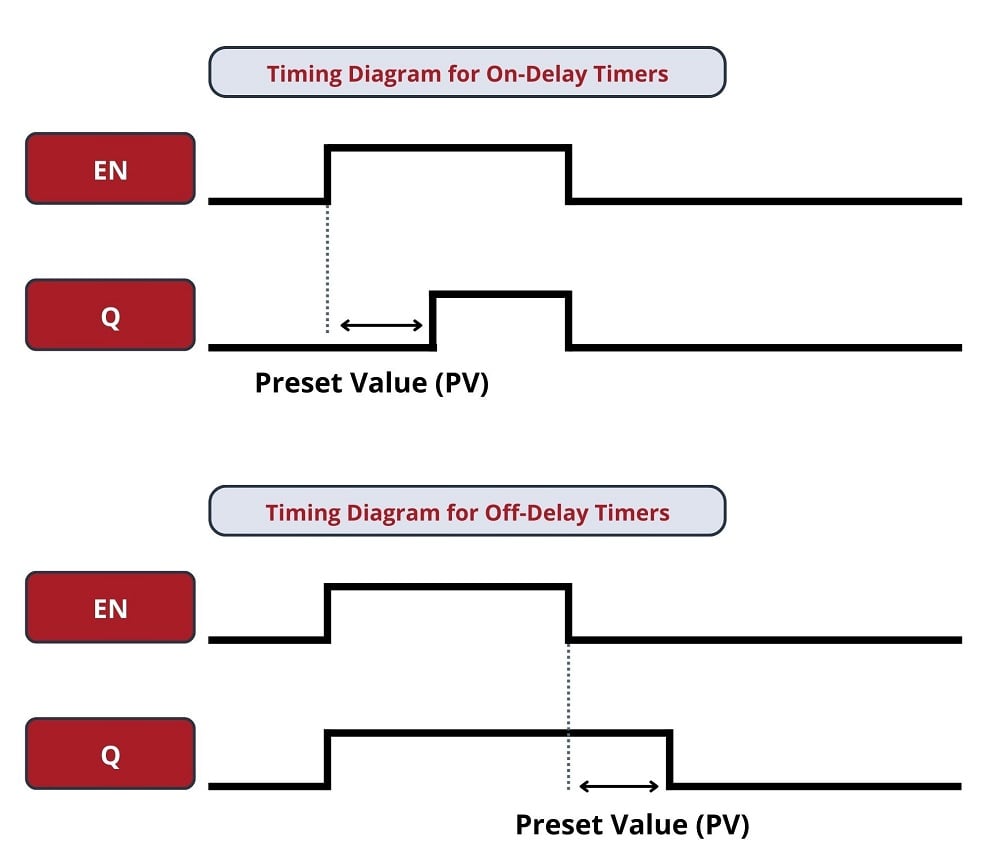
While it is common to find on-delay PLC instructions offered in both retentive and non-retentive forms within the instruction sets of nearly every PLC manufacturer and model, it is almost unheard of to find retentive off-delay timer instructions. Typically, off-delay timers are non-retentive only.
Ladder Logic Comparison Instructions
As we have seen with counter and timers, some PLC instructions generate digital values other than simple Boolean (on/off) signals. Counters have current value (CV) registers and timers have elapsed time (ACC) registers, both of which are typically double integer number values. Many other PLC instructions are designed to receive and manipulate non-Boolean values such as these to perform useful control functions.
The IEC 61131-3 standard specifies a variety of data comparison instructions for comparing two non-Boolean values and generating Boolean outputs. The basic comparative operations of “less than” (\(<\)), “greater than” (\(>\)), “less than or equal to” (\(\leq\)), “greater than or equal to” (\(\geq\)), “equal to” (=), and “not equal to” (\(\neq\)) may be found as a series of “box” instructions in the IEC standard:

The Q output for each instruction “box” activates whenever the evaluated comparison function is “true” and the enable input (EN) is active. If the enable input remains active but the comparison function is false, the Q output de-activates. If the enable input de-de-activates, the Q output retains its last state. The enable is shown above as a single N.O. contact on the left of each comparison instruction. If these are not included in the program, the comparison evaluation will be solely responsible for the output coil’s energized state.
A practical application for a comparative function is something called alternating motor control, where the run-times of two redundant electric motors are monitored, with the PLC determining which motor to turn on next based on which motor has run the least:


In this program, two retentive on-delay timers keep track of each electric motor’s total run time, storing the run time values in two registers in the PLC’s memory: RTO_1.CV and RTO_2.CV. These two integer values are input to the “greater than or equal to” instruction box for comparison. If motor 1 has run longer or equal to motor 2, the Mtr_1 bit will be latched on and motor 2 will be the one enabled to start up next time the “start” switch is pressed.
In the LES comparison, if motor 1 has run less time than motor 2, the Mtr_1 and Mtr_2 bits are reversed and motor 1 will be the one enabled to start. The two series-connected contacts Motor1 Out.2 and Motor2 Out.5 ensure the comparison between motor run times is not made until both motors are stopped. If the comparison were continually made, a situation might arise where both motors would start if someone happened to press the Start pushbutton while one motor is already running.
Ladder Logic Math Instructions
The IEC 61131-3 standard specifies several dedicated ladder instructions for performing arithmetic calculations. Some of them are shown here:

As with the data comparison instructions, each of these math instructions is optionally enabled by an “energized” signal to the enable (EN) input. Input and destination (output) values are linked to each math instruction by tag name.
An example showing the use of such instructions is shown here, converting a temperature measurement in units of degrees Fahrenheit to units of degrees Celsius. In this particular case, the program inputs a temperature measurement of 138 \(^{o}\)F and calculates the equivalent temperature of 58.89 \(^{o}\)C:

Note how two separate math instructions were required to perform this simple calculation, as well as a dedicated variable ('Extra_Float') used to store the intermediate calculation between the subtraction and the division “boxes.”
Although not specified in the IEC 61131-3 standard, many programmable logic controllers support Ladder Diagram math instructions allowing the direct entry of arbitrary equations. Rockwell (Allen-Bradley) RSLogix 5000 programming, for example, has the “Compute” (CPT) function, which allows any typed expression to be computed in a single instruction as opposed to using several dedicated math instructions such as “Add,” “Subtract,” etc. General-purpose math instructions dramatically shorten the length of a ladder program compared to the use of dedicated math instructions for any applications requiring non-trivial calculations.
For example, the same Fahrenheit-to-Celsius temperature conversion program implemented in RSLogix 5000 programming only requires a single math instruction and no declarations of intermediate variables:

"Drum" Sequencers
Many industrial processes require control actions to take place in certain, predefined sequences. Batch processes are perhaps the most striking example of this, where materials for making a batch must be loaded into the process vessels, parameters such as temperature and pressure-controlled during the batch processing, and then discharge of the product monitored and controlled. Before the advent of reliable programmable logic devices, this form of sequenced control was usually managed by an electromechanical device known as a drum sequencer. This device worked on the principle of a rotating cylinder (drum) equipped with tabs to actuate switches as the drum rotated into certain positions. If the drum rotated at a constant speed (turned by a clock motor), those switches would actuate according to a timed schedule.
The following photograph shows a drum sequencer with 30 switches. Numbered tabs on the circumference of the drum mark the drum’s rotary position in one of 24 increments. With this number of switches and tabs, the drum can control up to thirty discrete (on/off) devices over a series of twenty-four sequenced steps:

A typical application for a sequencer is to control a Clean In Place (CIP) system for a food processing vessel, where a process vessel must undergo a cleaning cycle to purge it of any biological matter between food processing cycles. The steps required to clean the vessel are well-defined and must always occur in the same sequence in order to ensure hygienic conditions. An example timing chart is shown here:

In this example, there are seven discrete outputs, one for each of the seven final control elements (pumps and valves). The process includes ten steps in sequence, each one of them is run for a pre-determined length of time. In this particular sequence, the only input is the discrete signal to commence the CIP cycle. From the initiation of the CIP to its conclusion several minutes or hours later, the sequencer simply steps through the programmed routine.
Another practical application for a sequencer is to implement a Burner Management System (BMS), also called a flame safety system. Here, the sequencer manages the safe start-up of a combustion burner: beginning by “purging” the combustion chamber with fresh air to sweep out any residual fuel vapors, waiting for the command to light the fire, energizing a spark ignition system on command, and then continuously monitoring for presence of good flame and proper fuel supply pressure once the burner is lit.
In a general sense, the operation of a drum sequencer is that of a state machine: the output of the system depends on the condition of the machine’s internal state (the drum position), not just the conditions of the input signals. Digital computers are very adept at implementing state functions, and so the general function of a drum sequencer should be (and is) easy to implement in a PLC. Other PLC functions we have seen (“latches” and timers in particular) are similar, in that the PLC’s output at any given time is a function of both its present input condition(s) and its past input condition(s). Sequencing functions expand upon this concept to define a much larger number of possible states (“positions” of a “drum”), some of which may even be timed.
Unfortunately, despite the utility of drum sequence functions and their ease of implementation in digital form, there seems to be very little standardization between PLC manufacturers regarding sequencing instructions. What follows here is an exploration of some different sequencer instructions offered by PLC manufacturers.
Click PLC Drum Instructions
The drum instruction offered in Koyo Click PLCs (manufactured by Automation Direct) is a model of simplicity itself. This instruction is practically self-explanatory, as shown in the following example:

The 8-by-5 grid of squares represent steps in the sequence and bit states for each step. Rows represent steps, while columns represent output bits written by the drum instruction. In this particular example, a five-step sequence proceeds at the command of a single input (Drum_Enable_Tag), and the drum instruction’s advance from one step to the next proceeds strictly on the basis of elapsed time (a time base orientation). When the input is active, the drum proceeds through its timed sequence. When the input is inactive, the drum halts wherever it left off, and resumes timing as soon as the input becomes active again.
Being based on time, each step in the drum instruction has a set time duration for completion. The first step in this particular example has a duration of 15 seconds, the second step 20 seconds, and the third step 10 seconds, and so on.
In the first step, output bits 1, 4, and 7 are set, corresponding to outputs Y000, Y003, and Y006.
In the second step, output bits 1, 3, 6, 7, and 8 are all set.
In the third step, output bits 1,2, 6, and 7 are set.
The highlighted versus blank boxes reveal which output bits are set and reset with each step. The current step number is held in a memory register DS1, while the elapsed time (in seconds) is stored in the timer register TD1. A “complete” bit is set at the conclusion of the three-step sequence.
Koyo drum instructions may be expanded to include more than three steps and more than three output bits, with each of those step times independently adjustable and each of the output bits arbitrarily assigned to any writable bit addresses in the PLC’s memory.
This next example of a Koyo drum instruction shows how it may be set up to trigger on events rather than on elapsed times. This orientation is called an event base:

Here, the five-step sequence proceeds when enabled by a single input (Drum_Enable_Tag), with the drum instruction’s advance from one step to the next proceeding only as the different event condition bits become set. When the input is active, the drum proceeds through its sequence when each event condition is met. When the input is inactive, the drum halts wherever it left off regardless of the event bit states.
For example, during the first step, the drum instruction waits for the first condition input bit X001 to become set (1) before proceeding to step 2, with time being irrelevant. When this happens, the drum immediately advances to step 2 and waits for input bit X002 to be set, and so forth. If multiple conditions were met simultaneously (X000, X001, and X002 for example all set to 1), the drum would skip through all steps as fast as it could (one step per PLC program scan) with no appreciable time elapsed for each step. Conversely, the drum instruction will wait as long as it must for the right condition to be met before advancing, whether that event takes place in milliseconds or in days.
Allen-Bradley Sequencer Instructions
Sequencer Output (SQO) Instruction
Rockwell (Allen-Bradley) PLCs use a more sophisticated set of instructions to implement sequences. The closest equivalent to Koyo’s drum instruction is the Allen-Bradley SQO (Sequencer Output) instruction, shown here:

You will notice there are no colored squares inside the SQO instruction box to specify when certain bits are set or reset throughout the sequence, in contrast to the simplicity of the Koyo PLC’s drum instruction. Instead, the Allen-Bradley SQO instruction is told to read a set of array data tags beginning at a location in the PLC’s memory specified by the programmer, one word or double word (DINT) at a time. It steps to the next word in that set of words with each new position (step) value. This means Allen-Bradley sequencer instructions rely on the programmer already having pre-loaded an area of the PLC’s memory with the necessary 1’s and 0’s defining the sequence. This makes the Allen-Bradley sequencer instruction more challenging for a novice programmer to interpret because the bit states are not explicitly shown inside the SQO instruction box, but it also makes the sequencer far more flexible in that these bits are not fixed parameters of the SQO instruction and therefore may be dynamically altered as the PLC runs.
With the Koyo drum instruction, the assigned output states are part of the instruction itself, and are therefore fixed once the program is downloaded to the PLC (i.e. they cannot be altered without editing and re-loading the PLC’s program). With the Allen-Bradley, the on-or-off bit states for the sequence may be freely altered during run-time. This is a very useful feature in recipe-control applications, where the recipe is subject to change at the whim of production personnel, and they would rather not have to rely on a technician or an engineer to re-program the PLC for each new recipe.
The “Length” parameter tells the SQO instruction how many words will be read (i.e. how many steps are in the entire sequence). The sequencer advances to each new position when its enabling input transitions from inactive to active (from “false” to “true”), just like a count-up (CTU) instruction increments its accumulator value with each new false-to-true transition of the input. Here we see another important difference between the Allen-Bradley SQO instruction and the Koyo drum instruction: the Allen-Bradley instruction is fundamentally event-driven, and does not proceed on its own like the Koyo drum instruction is able to when configured for a time base.
Sequencer instructions in Allen-Bradley PLCs use a notation called array indexed addressing to specify the locations in memory for the set of INTs or DINTs it will read. In the example shown above, we see the “Array” parameter specified as DINT_Array[0]. The “[0]” index symbol tells the instruction that this is a starting location in memory for the first 32-bit DINT, when the instruction’s position value is zero. As the position value increments, the SQO instruction reads array elements from successive addresses in the PLC’s memory. If DINT_Array[0] is the element referenced at position 0, then DINT_Array[1] will be the memory address read at position 1, DINT_Array[2] will be the memory address read at position 2, etc. Thus, the “position” value causes the SQO instruction to “point” or “index” to successive memory locations.
The bits read from each indexed word in the sequence are compared against a static mask specifying which bits in the indexed word are relevant. At each position, only these bits are written to the destination address.
To illustrate, let us examine a set of bits held in the B3 file of an Allen-Bradley ControlLogix or CompactLogix PLC, showing how each row (element) of this data file would be read by an SQO instruction as it stepped through its positions:

The sequencer’s position number is added to the file reference address as an offset. Thus, if the data file is specified in the SQO instruction box as DINT_Array[0], then DINT_Array[1] will be the row of bits read when the sequencer’s position value is 1, DINT_Array[2] will be the row of bits read when the position value is 2, and so on.
The mask value specified in the SQO instruction tells the instruction which bits out of each row will be copied to the destination address. A mask value of 16x FFFF FFFF (a full double integer filled with 1’s in hexadecimal format) means all 32 bits of each array element will be read and written to the destination. A mask value of 0000 0001 means only the first (least-significant) bit will be read and written, with the rest being ignored. If a bit has a 1 in the mask, the data will copy to the destination. A 0 in a bit will block the copy.
Let’s see what would happen with an SQO instruction having a mask value of FFFF FFFF, starting from file index DINT_Array[0], and writing to a destination that is output register Local:2:O.Data, given the bit array values in the array shown above. In this example, although the array is 32 bits in each DINT, only the lowest 16 of each DINT are displayed.

When this SQO instruction is at its third step position, it reads the bit values 1010 0111 from DINT_Array[2] and writes only those four bits to Local:2:O.Data. The “X” symbols shown in the illustration mean that all the other bits in that output register are untouched; the SQO instruction does not write to 0-masked bits because they are “masked off” from being written. You may think of the mask’s zero bits inhibiting source bits from being written to the destination word in the same sense that masking tape prevents paint from being applied to a surface.
The following Allen-Bradley RSLogix (Studio) 5000 PLC program shows how an SQO instructions plus an on-delay timer instruction may be used to duplicate the exact same functionality as the “time base” Koyo drum instruction presented earlier:

The first SQO instruction reads bits in the SEQ_Data_Array, sending them to the output register Remote:1:O.Data (the Mask tag value here is FFFF FFFF, so all data is copied).
A second array, called SEQ_Timing_Array, contains a list of the duration that each step should last. The MOV instruction reads the current step from the SEQ_Control position, and copies the time value from that array position into the timer’s preset.
The timer, in turn, is on a constant looping rotation, timing each of the specified delays and then incrementing the sequencer to advance to the next position when the time has elapsed.
Here we see a tremendous benefit of the SQO instruction’s indexed memory addressing: the fact that the SQO instruction reads its bits from arbitrarily-specified memory addresses means we may use SQO instructions to sequence any type of data existing in the PLC’s memory! We are not limited to turning on and off individual bits as we are with the Koyo drum instruction, but rather are free to index whole integer numbers, ASCII characters, or any other forms of binary data resident in the PLC’s memory.
Sequencer Compare (SQC) Instruction for SLC 500
Event-based transitions may be implemented in older Allen-Bradley PLCs (SLC 500 using RSLogix 500; this command does not exist in RSLogix 5000) using a complementary sequencing instruction called SQC (Sequencer Compare). The SQC instruction is set up very similar to the SQO instruction, except it does not contain a destination array to be written. Instead, it contains a reference array against which the data array is compared
This can be useful when comparing the current input register of a module (16 bits in the SLC 500 structure) against a pre-defined 16-bit word. If the input conditions match, an FD (Found) bit is set, which can be used to increment the SQC instruction.
Sequencer Load (SQL) Instruction
Lastly, Allen-Bradley PLCs offer a third sequencing instruction called Sequencer Load (SQL), which performs the opposite function as the Sequencer Output (SQO). An SQL instruction takes data from a designated source and writes it into an indexed register according to a position count value, rather than reading data from an indexed register and sending it to a designated destination as does the SQO instruction. SQL instructions are useful for reading data from a live process and storing it in different registers within the PLC’s memory at different times, such as when a PLC is used for datalogging (recording process data).
REVIEW:
-
Counters and timers are simple structures that require an input to trigger the enable, and an output that changes at the end of the timing or counting preset value.
-
Comparison contacts provide a way to compare two integers or real data types and provide an on/off Q output.
-
Math commands use two or more input variables, perform an instruction, and save the new value to a destination. Custom math expressions can be created.
-
Sequencers can provide step-by-step process execution using predefined times, or by using events to drive systematic operations.
Interested in more PLC content?
Related Videos:
Textbook Pages:
Tutorials and Technical Articles:
- Ladder Logic in Programmable Logic Controllers (PLCs)
- Intro to PLC Programming with Rockwell’s Studio 5000 and CompactLogix
- Intro to Siemens S7-1200 PLC and TIA Portal Programming
- Understanding PLC Program Commands: Timers
