How Does Motion Planning for Autonomous Robot Manipulation Work?

Autonomous manipulation in static and dynamic environments — as well as structured and unstructured environments — have their own technical challenges and applications. Industrial autonomous manipulation uses visual servoing and motion planning to control the motion of the robot using online perception for environment updates or assuming the environment being controlled.

This article discusses the technical aspects of the motion planning pipeline for the autonomous operation of robot manipulators and how they are applied in the industry.

 

What is Motion Planning?

Motion planning is the technique of determining the path and motion characteristics for autonomous robot motion for any task. Path planning defines the route that the robot takes to go from point A to point B, while motion planning includes the motion profile, i.e., the temporal sequence of positions, velocities, and accelerations for the robot motion along with other environmental considerations. Motion planning is possible in both task space and configuration space.

 

Figure 1. Motion path for a mobile robot

 

Path planning algorithms for task space usually define the route for the center of the robot, agnostic to the robot type and ignorant of the robot kinematics and dynamics. Motion planning involves broader considerations around:

• motion quality
• reactive planning
• dynamic environment management
• kinodynamic robot constraints
• high-dimensional planning
• velocity profiling
• robot dimensions/footprint. 

Motion planning solutions address four blanket domains depending on the robot environment, the problem formulation, its computational representation, and the environment map. It includes planning under different system constraints, discrete space planning (where the achievable task space configurations are finite and predefined), continuous space planning, and planning in uncertainty.

 

Configuration Space for Manipulators

The configuration space of a manipulator is the collection of all the possible combinations of the positions of joints, revolute, or prismatic that the robot can achieve. A lot of the is impossible for the robot to achieve and is called due to self-collision (the robot collides with itself) or collision with the world elements while the free space is called .

It is essentially a vector of the positions of the joints = [q1, q2, q3, q4, q5]. The task space for the manipulator end-effector is the collection of 3D Cartesian poses (position and orientation)

 

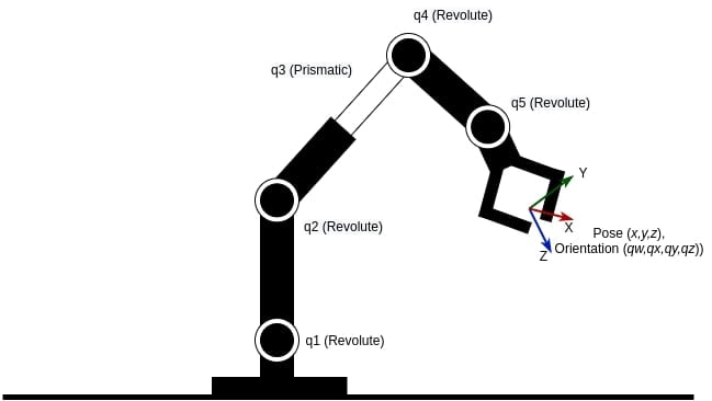
Figure 2. Robot Manipulator Cspace and task space

 

Motion Planning for Manipulators

The motion planning problem for manipulators can be formulated as finding a continuous path for or in task space.

 

Figure 3. Robot Manipulator Motion Planning Visualization

 

As mentioned above regarding the motion planning paradigms, planning for manipulators can be done in discrete space (by representing the task space as a set of connected graph points where points are centers of grids from cellular decomposition) or in the continuous space where the complete task space is used to find the solution by searching for a feasible path through it.

 

Challenges of Motion Planning for Manipulators

Manipulators have an intricate design and the planning solutions have a lot of constraints to handle and limitations to work with in real-time  in order to generate reliable solutions. Common challenges include:

1. The high-dimensional Cspacefor high-DOF robot arms introduce lots of possible configurations of the kinematic chain. Planning in the task space and then executing the motion in Cspace is extremely challenging due to collisions and feasibility challenges. 
2. Velocity profile generation while obeying boundary conditions, constraints for high-order motion terms (velocity, acceleration, and jerk) and satisfying motion quality requirements is difficult.
3. Online inverse kinematics solutions while dealing with singularities and low manipulability zones for executing motion in real-time is difficult.
4. Position and orientation limits for the end-effector can narrow down the task space available for solutions.
5. Joint limits and DOFs can narrow the Cspaceand the feasibility of task-space solutions converted into Cspace
6. Getting planning solutions while managing the computational resources is also challenging.

 

Motion Planning Configuration Elements

The motion planning pipeline needs to be configured before it starts finding solutions. These specifications are a mix of robot-related variables, the configurable software tools, and the environment.

1. The geometric description of the robot (usually a lot of the tools and software prefer the URDF robot model) is needed. This is used to derive the kinematic chain for forward/inverse kinematics and the collision tags are used to derive the 3D model geometry to run collision checks. 
2. The geometric description of the world is enclosed in the map and updated as per the environment behavior, static or dynamic.
3. User-defined allowed collision matrix defines robot-link - robot-link or robot-link - world elements that should not be checked for collision due to low possibility or infeasibility. For example, the base link of the robot should not be checked for collision against the mounting platform, and collision checking for two consecutive robot links is usually not needed as they cannot physically intersect unless they have special intricate designs.
4. The motion planning framework needs kinematic solvers to toggle between task space and joint space. Several off-the-shelf inverse kinematics solvers are readily available as plugins to be used in larger motion planning frameworks. 
5. Velocity profile parameters like velocity, acceleration, and jerk limits and the type of profile to be used are configured for the planning pipeline.

 

Motion Planning Pipeline for Manipulators

The motion planning pipeline involves elements from the robot environment, the robot’s own motion strategy, and the computational aspects of processing all the required algorithms. The pipeline can be seen below in Figure 4.

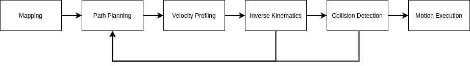
Figure 4. The motion planning pipeline elements 

   

The most important nuances of obtaining motion planning solutions for manipulators (considering the solution in task space) includes:

1. Environmental mapping
2. Planning
3. Velocity profiling
4. Inverse kinematics
5. Collision Detection
6. Motion Execution

 

Environment Mapping

The robot environment can be occupied by external elements and thus not navigable. Hence, mapping is critical to define the free task-space available for planning in a dynamic environment. For fixed-based manipulators, 3D occupancy grids are the most suitable mapping technique. More about them can be found in the SLAM article series.

 

Planning

Planning is, unsurprisingly, the most important part of motion planning. It involves determining a feasible and optimized path through the environment from the start to the goal point. The path consists of a sequence of poses, whereas its extension to a trajectory means additional information with the desired temporal distribution of velocities and accelerations for the end-effector, considering the various constraints discussed above. More about planning algorithms are discussed below.

Very often path optimization methods are used to enhance the quality of the path and avoid jerks or kinks, while optimizing the paths around multivariate objective (low energy and less motion time) functions. 

 

Velocity Profiling

Motion profiles define the variation of the velocity of a point (here the manipulator end-effector), between any two points. After  a path is obtained, motion profiles decide how the end-effector should move while satisfying all the boundary conditions and trajectory requirements along with ensuring smooth motion. 

The most common velocity profile used is the trapezoidal profile, easy to program but has a lot of instantaneous acceleration changes and impulsive jerks — not the smoothest for highly dynamic robots. The S-curve profile is a smoother profile that accelerates and decelerates the robot gradually when waking up from rest, thus ensuring smoother motion.

 

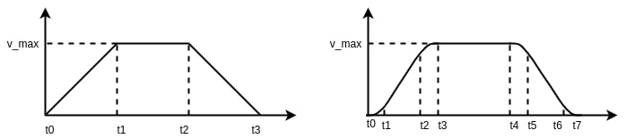
Figure 5. Trapezoidal Profile vs S-Curve 

 

Inverse Kinematics 

After the velocity profiles generate the next target pose (profiles generate instantaneous target velocity but a controller needs the next interpolated position derived from the instantaneous velocity), usually in the task space to execute the motion, real-time inverse kinematics solutions to generate joint angle instructions for the manipulator joints.

 

Collision Detection

Collision detection involves representing the robot links and other real-world objects as polygonal shapes or meshes occupying space in the 3D world and comparing to see if any two of them intersect/overlap or not. The axis-aligned bounding box (AABB) and oriented bounding box (OBB) are the most common coarse polygonal representations of the robot. The Gilbert-Johnson-Keerthi (GJK) distance algorithm is one of the most used collision detection algorithms. 

If the next target joint position vector isn’t feasible because it can cause collisions (self or robot with the world), a recovery plan is run which may include  rerunning the planning algorithm for new path solutions or tweaking the next move and retrying. This is the most time-consuming step, thus a lot of motion planning is preempted to avoid runtime computational load for this step.

 

Motion Execution

The final step of the pipeline is executing the joint instruction using conventional position-control (conventional PD + gravity compensation) or hybrid position-force control or other methods.

 

Motion Planning Algorithms

Planning algorithms are broadly classified into search-based discrete planners or sampling-based algorithms. 

Search-based algorithms are employed in discrete environments where paths are derived from a connected graph that has a path from the start to the target point. Common search-based algorithms are usually graph-search algorithms like breadth-first search (BFS), depth-first search (DFS), A* and Dijkstra. BFS and DFS are uninformed searches ignorant to the cost of traversing the different edges of the graph, usually very inefficient, and not practically deployable in large-scale applications.

A* and Dijkstra’s algorithms are greedy searches that use an immediate reward and a heuristic to compute the best next position to go to. A heuristic is the best “guesstimate” of the cost to move from the current node to the target. An admissible heuristic ensures that the predicted cost is always less than or equal to the actual cost and helps drive the search correctly (only for A* search). While the Dijkstra’s algorithm only uses the greediest next step, A* uses the next cost as well as the heuristic.

 

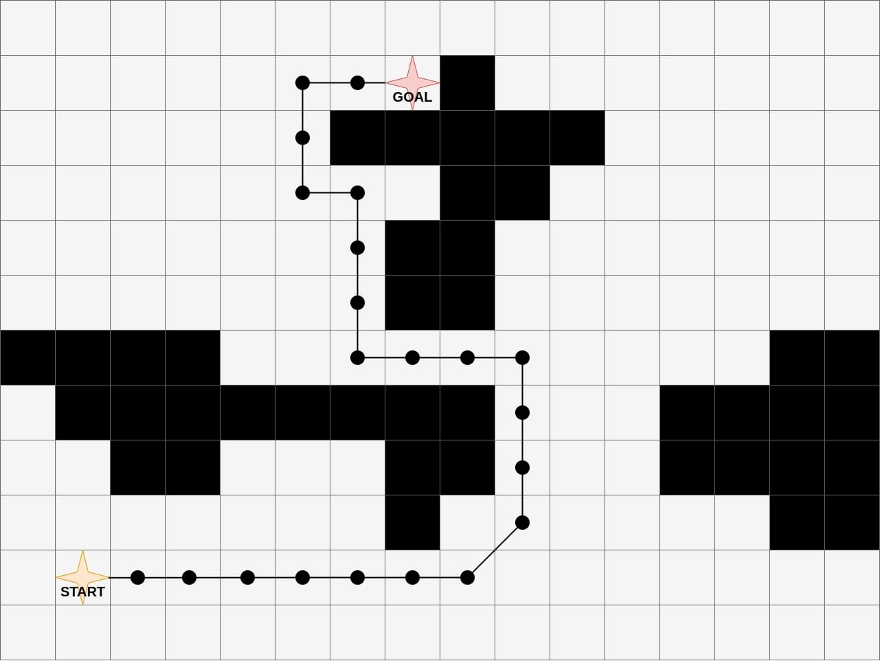
Figure 6. A* pathfinding algorithm 

 

Rapidly-exploring random trees (RRT) and probabilistic roadmaps (PRM) are the most common sampling-based algorithms that randomly extract path points from the continuous 3D coordinates and derive a path through it. RRT*, RRTConnect, and bidirectional RRT are enhancements to the original RRT algorithm used due to improved run-time performance and path continuity.

 

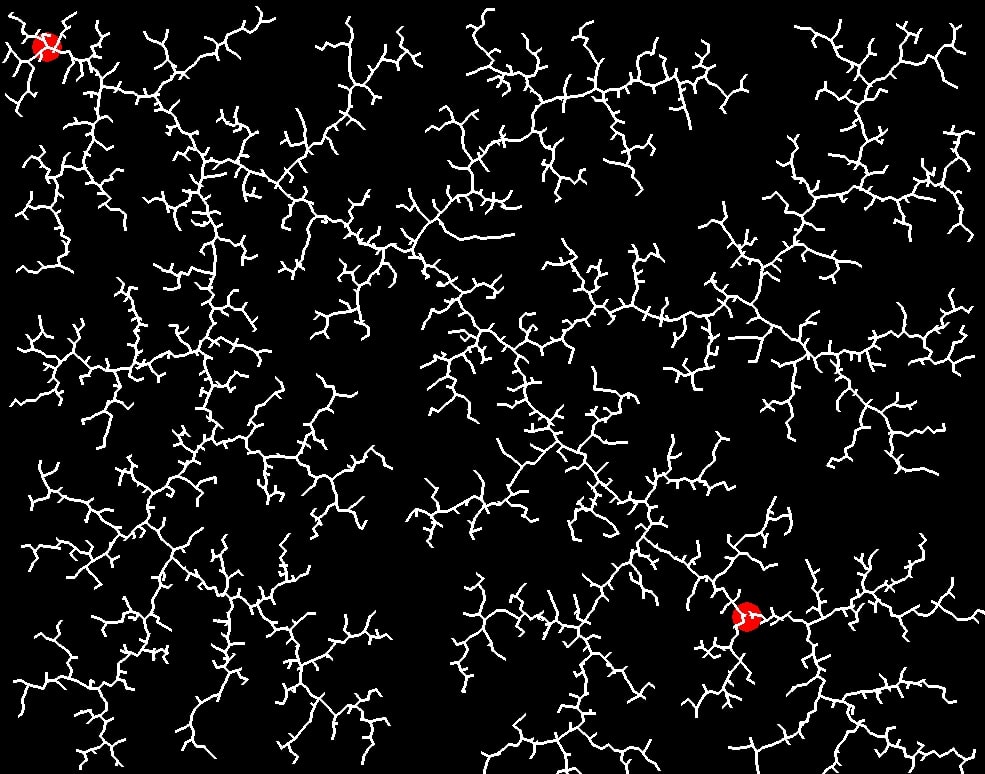
Figure 7. RRT Algorithm 

 

Common, widely-used planning libraries include the Open Motion Planning Library (OMPL), Search-Based Planning Library, and Covariant Hamiltonian Optimization (CHOMP) with implementations for multiple search-based, sampling-based, and hybrid motion planning algorithms. 

 

Motion Planning In Commercial Applications

Realtime autonomous manipulation applications in factories are usually limited to controlled environments with the least expectations of human intervention or mishaps.  A common example is a robot workcell, an enclosed and isolated area for the robot to work in. Robotic welding and soldering use considerable motion planning to design the correct robot path for operation.

Pick-and-place is the most common application where the robot grabs an object, and autonomously creates a path to the target drop point. Packaging, sorting, palletizing, and device testing applications are built on top of this.

A lot more motion planning is used in semi-structured environments like warehouses where manipulators fetch objects from shelves and drop them at desired locations. Inventory management and stock replenishment applications are being explored in a limited capacity but heavily use motion planning.

 

Review Of Motion Planning

Realtime motion planning has two major bottlenecks: computationally expensive (due to collision checking, inverse kinematics, and perception) and lack of robustness (multiple IK solutions and different path possibilities). These bottlenecks limit their extensive use in high-performance requirement areas. The advent of deep learning and GPUs has  brought new hopes for the near future.

The previous article on visual serving and this motion planning article lay the foundation for the next article on the automated bin-picking application design and implementation in a commercial setting.