Motion Control Tutorial: Cyclic Actions Using the Record Table

Previously, we set up a motion axis and jogged it using the simple interface provided by Festo’s Automation Suite configuration and plug-in control software.

The next step is to arrange a basic sequence of motion commands in what Festo calls a "record table." A sequencing instruction set requires two elements. First, we must define each action (usually an absolute or incremental position reference). Then we need to define transition events that determine when each action ends and the next one begins.

 

Figure 1. Ball-screw axis with direct-mount motor.

 

Record Table Motion

For many simple applications, the motion is really just a repetition of two or three commands over and over again in a cycle. We can arrange these very easily in the Record table.

Open a recent project in Festo’s Automation Suite, such as the one we created in our first tutorial.

Navigate to the parameterization tab, expand Axis 1 on the left, and click “Record Table.” Add a record set with a target position near the far end of your axis, which is 350 mm for me. Add a second record with a target close to the motor end, perhaps around 50 mm. You might also want to decrease the default velocity when getting started with motion, or you might be in for a surprise.

 

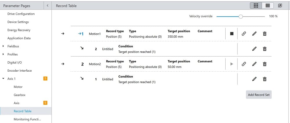
Figure 2. Record table showing two motion record sets.

 

Note: You can view and play the record instructions from the control tab, but you must be in the parameterization tab to create and edit the records.

This isn’t limited to simply a "bench test" proof of concept for motion control. These record sets can also be controlled and run by a PLC, which means that you can build a complex instruction set for real-world systems that considers more than just position and velocity.

Acceleration and deceleration are important for high-mass or liquid products that may cause instability if the velocity changes too quickly. Jerk is another motion term that is a bit harder to understand, but just as acceleration is a change in velocity over a short time, jerk is the change in acceleration over a short time.

 

Linking Records

Next, we need to determine when each motion command starts. Most often, this will happen just after a previous command is finished or after a digital input (like a proximity sensor) is energized, but there are many ways to trigger a transition.

For each record, press the chain link button, which will open up the transition menu. Again, there are many ways to trigger the transition, but let’s discuss some of the most common:

• Target Position Reached: The encoder tracks the actual position. This is good for moves without any changing resistance, like a robot on a 7th axis (constant load mass is fine).
• Target Torque Reached: The motor current is used to monitor a clamping force, and it will stop (without faulting, thank goodness) when a torque is reached–useful for moves with variable-sized loads or positions.
• Time: a simple timer, but useful for processes that must have a specified duration. DO NOT use a timer to compensate for inaccurate process variables like friction or upstream delays.
• Digital Input: This provides flexibility for any digital or legacy system, like a robot or a sensor. Don’t have any advanced COM protocol? No problem, use a digital signal.

For our project, we will link according to the target position so that we are isolated from any external factors. When the record target position is reached, link to the second record. Likewise, when the second record position is reached, link to the first record. This will create an infinite cycle.

 

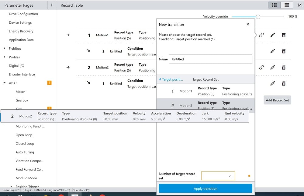
Figure 3. Adding transitions to step between the motion record sets.

 

Restart the device and save the changes. In the "Control" tab, enable the Plug-in and Powerstage. Finally, access the Record Table and play the first record using the triangle play button. Watch it carefully, and be ready to press the stop button if it’s about to collide, but if all is well, your axis should be moving back and forth!

 

A Bit About Monitoring

These days, we can get nearly any data into the cloud and display it on a dashboard. But when we are working with standalone, isolated systems, it’s helpful to have a way to monitor important factors within that system.

In the Festo Automation Suite, we can view the target and actual positions, currents, velocities, and controller signals very easily. This ability is called "tracing," and it’s activated by triggers within the software commands or within the axis itself.

When recording a trace, we can set the time before and after a trigger to display, giving us insight into what may have happened moments before an event, like a communication or overcurrent error.

Since we don’t expect any errors on our bench setup, we’ll set up a simple test record trace that will provide a log when the velocity increases above a specific threshold.

Navigate to the Diagnostics tab and enter Trace Configuration. There are many plot channels already active (like a multi-channel oscilloscope), but they can show nearly any data you could wish! Velocity, current, commanded position, actual position, acceleration, and even config parameters.

 

Trace Channels

Let’s uncheck all channels except setpoint position, actual position, and actual velocity. The others are fine, but more channels make the plot harder to read.

 

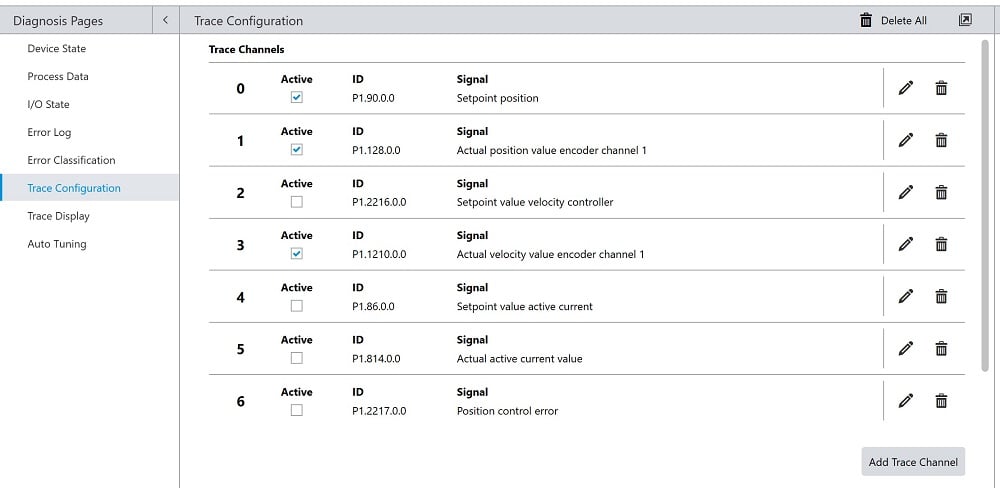
Figure 4. We are choosing to view only the setpoint, current position, and current velocity.

 

Trace Duration

Next, we determine the total length of the recording snapshot. Note: this is not an ongoing live read-out; this will create a fixed image that lasts for the duration specified in the "Trace Duration" box. I will leave the default of ~1.6 seconds.

 

Trigger Settings

Finally, the Trigger configuration consists of determining what factor is supposed to tell the computer to save and display the snapshot. For this demo, I will choose to get a recording when the velocity rises above 10 mm/sec (you could choose any low value that we are sure to cross).

I will use the common data trigger of “P1.2216.0.0 Setpoint value velocity controller” with a rising edge threshold of 0.01 m/s.

The trace delay is the number of seconds before the event that will be captured and displayed. The total trace duration then is the addition of the trace delay plus the duration after the trigger. I’ll choose 1.2 seconds of trace delay, which means I will also have 0.4 seconds of trace after the trigger event.

 

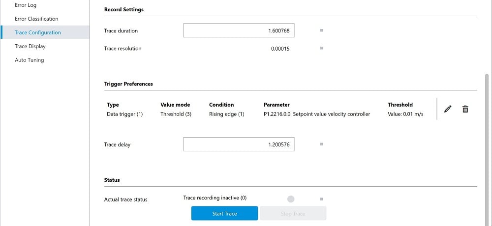
Figure 5. Adding the trigger parameter and starting the trace.

 

Start and View The Trace

Press the Start Trace button at the bottom to begin monitoring for the trigger event. Once the motion carriage reaches the motor end, then turns around and reverses direction to positive, you will be alerted that a new trace is recorded and is seen in the Trace Display tab on the left.

In this tab, you’ll see the plot with a timestamp, the various chosen channels (for which visibility can be individually toggled), and tools to investigate and save the plot as a decently high-res PNG.

 

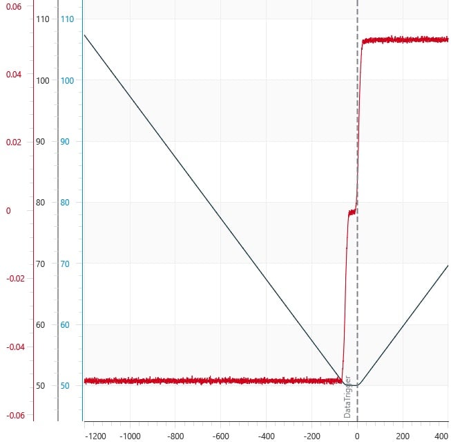
Figure 6. The final plot shows 1.2 seconds (1200 ms) before the trigger and 0.4 seconds after. The gray line shows the current position (superimposed over the blue line, the target position) and the velocity in red. The velocity is steady at -0.05 m/s, then drops to zero with a high deceleration rate, then rises with a high acceleration rate to a constant 0.05 m/s.

 

What’s Next for Motion?

The next step in complexity is to drive motion commands from an external controller, like a PLC. In the next article, we will set up a simple program that removes the need for the laptop in the control loop, acting more like a standalone automated process.

 

All images used courtesy of the author