 Facebook
 Google
 GitHub
 Linkedin
Chromatography: Methods, Detectors and Species
Imagine a major marathon race, where hundreds of runners gather in one place to compete. When the starting gun is fired, all the runners begin running the race, starting from the same location (the starting line) at the same time. As the race progresses, the faster runners distance themselves from the slower runners, resulting in a dispersion of runners along the race course over time.
Now imagine a marathon race where certain runners share the exact same running speeds. Suppose a group of runners in this marathon all run at exactly 8 miles per hour (MPH), while another group of runners in the race run a bit slower at exactly 6 miles per hour, and another group of runners plod along at exactly 5 miles per hour. What would happen to these three groups of runners over time, supposing they all begin the race at the same location and at the exact same time?
As you can probably imagine, the runners within each speed group will stay with each other throughout the race, with the three groups becoming further spread apart over time. The first of these three groups to cross the finish line will be the 8 MPH runners, followed by the 6 MPH runners a bit later, and then followed by the 5 MPH runners after that. To an observer at the very start of the race, it would be difficult to tell exactly how many 6 MPH runners there were in the crowd, but to an observer at the finish line with a stop watch, it would be very easy to tell how many 6 MPH runners competed in the race, by counting how many runners crossed the finish line as a distinct group at the exact time corresponding to a speed of 6 MPH.
Now imagine a mixture of chemicals in a fluid state traveling through a very small-diameter “capillary” tube filled with an inert, porous material such as sand. Some of those fluid molecules will progress more easily down the length of the tube than others, with similar molecules sharing similar propagation speeds. Thus, a small sample of that chemical mixture injected into such a capillary tube, and carried along the tube by a continuous flow of solvent (gas or liquid), will tend to separate into its constituent components (called species) over time just like the crowd of marathon runners separate over time according to running speed. Slower-moving molecules will experience greater retention time inside the capillary tube, while faster-moving molecules experience less. A detector placed at the outlet of the capillary tube, configured to detect any chemical different from the solvent, will indicate the different species exiting the tube at different times. If the retention time of each chemical species is known from prior tests, this device may be used to identify the composition of the original chemical mix (and even how much of each species was present in the injected sample) based solely on the time delay of each species exiting the column. More importantly, this one device will be able to identify and quantify a great many chemical compounds present in the original sample, a feat unmatched by most analytical technologies.
This is the essence of chromatography: the technique of chemical separation by time-delayed travel down the length of a stationary medium (called a column). In chromatography, the chemical solution traveling down the column is called the mobile phase, while the solid and/or liquid substance residing within the column is called the stationary phase. Chromatography was first applied to chemical analysis by a Russian botanist named Mikhail Tswett, who was interested in separating mixtures of plant pigments. The colorful bands left behind in the stationary phase by the separated pigments gave rise to the name “chromatography,” which literally means “color writing.”
Modern chemists often apply chromatographic techniques in the laboratory to purify chemical samples, and/or to measure the concentrations of different chemical substances within mixtures. Some of these techniques are manual (such as in the case of thin-layer chromatography, where liquid solvents carry liquid chemical mixtures along a flat plate covered with an inert coating such as alumina, and the positions of the chemical drops after time distinguishes one chemical species from another). Other techniques are automated, with machines called chromatographs performing the timed analysis of chemical travel through tightly-packed tubular columns. The main focus of this section will be automated chromatography, as is used for continuous process analysis.
Manual chromatography methods
One of the manual chromatography methods taught to beginning chemists is thin-layer chromatography, also known as TLC. An illustrated sequence showing thin-layer chromatography appears here:

The simplest forms of chromatography reveal the chemical composition of the analyzed mixture as residue retained by the stationary phase. In the case of thin-layer chromatography, the different liquid compounds of the mobile phase remain embedded in the stationary phase at distinct locations after sufficient “developing” time. The same is true in paper-strip chromatography where a simple strip of filter paper serves as the stationary phase through which the mobile phase (liquid sample and solvent) travels: the different species of the sample remain in the paper as residue, their relative positions along the paper’s length indicating their extent of travel during the test period. If the chemical species happen to have different colors, the result will be a stratified pattern of colors on the paper strip.
Automated chromatographs
The most common type of chromatography used in continuous process analysis is the gas chromatograph (abbreviated “GC”), so named because the mobile phase is a gas (or a vapor rather than a liquid. In a GC, the sample to be analyzed is injected at the head of a very long and very narrow tube packed with solid and/or liquid material. This long and narrow tube (called the column) is designed to impede the passage of the sample molecules. A continuous flow of “carrier gas” washes the sample compounds down the length of the column, allowing them to separate over time according to how they interact with the stationary phase packed inside the column. A simplified schematic of a process GC shows how it functions:

The sample valve periodically injects a very precise quantity of sample into the entrance of the column tube and then shuts off to allow the constant-flow carrier gas to wash this sample through the length of the column tube. Each chemical species within the sample travels through the column at different rates, exiting the column at different times. All the detector needs to do is be able to tell the difference between pure carrier gas and carrier gas mixed with anything else.
An important detail to note here is that the detector need not be discriminatory in its response to different chemical compounds, with just one exception: it need only distinguish between carrier and non-carrier compounds. The ability for an analyzer to measure singular compounds out of a mixture is the fundamental challenge of all analytical instrumentation, and here we see the genius of chromatography: the variable we use to discriminate between different chemical compounds within the sample is retention time through the column and nothing else. Rather than rely on some clever sensor technology to selectively detect one chemical compound out of a mixture, we are able to use a non-specific sensor and let time be the discriminating variable.
Appealing to the marathon analogy again, it’s as if a platform weigh-scale is situated at the finish line, to weigh the runners as they finish the race. The scale cannot discern the running speed of any runner by their measured weight – indeed, all the scale indicates is that someone is crossing the finish line – but it can determine the running speed based on when the runner steps on the scale.
If we plot the response of a chromatograph’s detector on a graph, we see a pattern of peaks, each one indicating the departure of a species “group” (i.e. a different chemical compound) exiting the column. This graph is typically called a chromatogram:

Narrow peaks represent compact bunches of molecules all exiting the column at nearly the same time, analogous to a group of runners crossing the finish line running shoulder-to-shoulder, all stepping on and off the platform scale at the same time. Wide peaks represent more diffuse groupings of similar (or identical) molecules, analogous to a group of equally-fast runners crossing the finish line as a diffuse group. In this chromatogram, you can see that species 4 and 5 are not clearly differentiated over time. Better separation of species may be achieved by altering the sample volume, carrier gas flow rate, carrier gas pressure, type of carrier gas, column packing material, and/or column temperature.
Species identification
Recall that the purpose of any analytical instrument is to discriminately measure one variable or component concentration amongst a mix of different chemical components. The fundamental challenge of chemical analysis is how to reliably and accurately detect that one “species” of chemical while being unaffected by the presence of any other chemical species. Most analyzers rely on a sensor that exploits some unique characteristic of the chemical of interest (e.g. its unique ability to pass through a special membrane, its ability to absorb a unique spectrum of light, its tendency to engage in a unique chemical reaction, etc.), but not chromatographs. Chromatographs simply delay the flow rate of different chemical species through a long tube based on those species’ mass and interactions with the stationary phase, using time as the discriminating variable. This allows chromatographs to be nearly universal in the range of chemical species they can measure while using relatively simple and uncomplicated detectors. The detector need only discriminate between carrier gas and anything that isn’t carrier gas in order to serve its purpose in a gas chromatograph. Identifying a suitable detector technology is relatively easy given the fact that the type of carrier gas used in a GC is something chosen by the designer of the GC. In other words, chromatography gives one the freedom to choose a compound that’s easy for a sensor to detect, rather than try to find a sensor able to detect the specific species one needs to measure in the process. This is important given the fact that there are many more types of chemical compounds in the world than there are chemical sensor types!
In general, chemical compounds having less molecular weight tend to exit the column earlier, while compounds having greater molecular weight exit the column later. The precise sequence of species elution through a column depends greatly on the stationary phase material type, as well as the carrier fluid type. Proper selection of stationary phase and carrier compounds is essential to efficient chromatograph operation, and is usually the domain of trained chemists.
To view a flip-book animation showing how a chromatograph separates a sample into its constituent species, turn to Appendix 35.6 beginning on page .
Since species identification in a chromatograph is performed with time as the discriminating factor, a chromatograph’s ability to accurately identify chemical compounds depends on its control computer “knowing” when to expect various compounds to exit the column. Chromatographs are calibrated by injecting a sample containing known concentrations of the species of interest (as well as any potentially interfering species), then timing the beginnings and ends of each species peak as each substance exits the column.
Chromatograph detectors
Several different detector designs exist for process gas chromatographs. The two most common are the flame ionization detector (FID) and the thermal conductivity detector (TCD). Other detector types include the flame photometric detector (FPD), photoionization detector (PID), nitrogen-phosphorus detector (NPD), and electron capture detector (ECD). All chromatograph detectors exploit some physical difference between the solutes and the carrier gas itself which acts as a gaseous solvent, so that the detector may be able to detect the passage of solute molecules among carrier molecules.
Flame ionization detectors work on the principle of ions liberated in the combustion of the sample species. Here, the assumption is that sample compounds will ionize inside of a flame, whereas the carrier gas will not. A permanent flame (usually fueled by hydrogen gas which produces negligible ions in combustion) serves to ionize any gas molecules exiting the chromatograph column that are not carrier gas. Common carrier gases used with FID sensors are helium and nitrogen, which also produce negligible ions in a flame. Molecules of sample encountering the flame ionize, causing the flame to become more electrically conductive than it was with only hydrogen and carrier gas. This conductivity causes the detector circuit to respond with a measurable electrical signal. A simplified diagram of an FID is shown here:

Hydrocarbon molecules happen to easily ionize during combustion, which makes the FID sensor well-suited for GC analysis in the petrochemical industries where hydrocarbon composition is the most common form of analytical measurement. It should be noted, however, that not all carbon-containing compounds significantly ionize in a flame. Examples of non-ionizing organic compounds include carbon monoxide, carbon dioxide, and carbon sulfide. Other gases of common industrial interest such as water, hydrogen sulfide, sulfur dioxide, and ammonia likewise fail to ionize in a flame and thus are undetectable using an FID.
Thermal conductivity detectors work on the principle of heat transfer by convection (gas cooling). Here, the assumption is that sample compounds will have different thermal properties than the carrier gas. Recall the dependence of a thermal mass flowmeter’s calibration on the specific heat value of the gas being measured. This dependence upon specific heat meant that we needed to know the specific heat value of the gas whose flow we intend to measure, or else the flowmeter’s calibration would be in jeopardy. Here, in the context of chromatograph detectors, we exploit the impact specific heat value has on thermal convection, using this principle to detect compositional change for a constant-flow gas rate. The temperature change of a heated RTD or thermistor caused by exposure to a gas mixture with changing specific heat value indicates when a new sample species exits the chromatograph column.
A simplified diagram of a TCD is shown here, with pure carrier gas cooling two of the self-heated thermal sensors and sample gas (mixed with a carrier gas, coming off the end of the column) cooling the other two self-heated sensors. Differences in thermal conductivity between gas exiting the column versus pure carrier gas will cause the bridge circuit to unbalance, generating a voltage signal at the output of the operational amplifier circuit:

This type of chromatograph detector works best, of course, when the carrier gas has a significantly different specific heat value than any of the sample compounds. For this reason, hydrogen or helium (both gases having very high specific heat values compared to other gases) are the preferred carrier gases for chromatographs using thermal conductivity detectors.
Measuring species concentration
While time is the variable used by a chromatograph to discriminate between different species (types) of chemical compounds, the concentration (quantity) of each chemical compound in the sample is inferred from the magnitude of the detector’s response as it senses each compound. Specifically, the quantity of each species present in the sample may be determined by applying the calculus technique of integration to each chromatogram peak, calculating the area underneath each curve. The vertical axis represents detector signal strength, which is proportional to the rate at which detected molecules are flowing through the sensor at any given time. This means the height of each peak represents the mass flow rate of each species (\(W\), in units of micrograms per minute, or some similar units) passing through the detector. The horizontal axis represents time, so, therefore, the integral (sum of infinitesimal products) of the detector signal over the time interval for any specific peak (time \(t_1\) to \(t_2\)) represents a mass quantity that has passed through the column. In simplified terms, a mass flow rate (micrograms per minute) multiplied by a time interval (minutes) equals mass in micrograms:
\[m = \int_{t_1}^{t_2} W \> dt\]
Where,
\(m\) = Mass of sample species in micrograms
\(W\) = Instantaneous mass flow rate of sample species in micrograms per minute
\(t\) = Time in minutes (\(t_1\) and \(t_2\) are the interval times between which total mass is calculated)
As is the case with all examples of integration, the unit of measurement for the totalized result is the product of the units within the integrand: flow rate (\(W\)) in units of micrograms per minute multiplied by increments of time (\(dt\)) in the unit of minutes, summed together over an interval (\(\int_{t_1}^{t_2}\)), result in a mass quantity (\(m\)) expressed in the unit of micrograms. Integration is really nothing more than the sum of products, with dimensional analysis working as it does with any product of two physical quantities:
\[\left({[\mu \hbox{g}] \over [\hbox{min}]}\right) [\hbox{min}] = [\mu \hbox{g}]\]
This mathematical relationship may be seen in graphical form by shading the area underneath the peak of a chromatogram:

Returning to the marathon analogy again, imagine the platform scale at the finish line being the detector, the racecourse is the chromatography column, and the runners being individual molecules (each type of molecule running at its own unique speed). If we wish to quantify how many runners of a certain speed were in the race, we would need to integrate the scale’s weight reading during the time period in which we expect that class of runners to arrive at the finish line. If a group of runners crosses side-by-side such that they all step on the scale and leave the scale simultaneously, the scale’s indication will be a tall and narrow peak when plotted on a time-based graph. If an identical-size group of runners arrives at the finish line at some other time, but cross in single-file form rather than side-by-side, the scale will register each runner’s weight one at a time with the graphed response being a much shorter and much wider peak. In either group, though, it’s the same number of runners finishing. Therefore both the height of the peak (i.e. scale weight) and the duration of the peak need to be taken into consideration when calculating how many runners were in a particular group.
Precise quantitative measurement of species concentration, however, is a bit more complicated than simply integrating detector peaks over time. A problem we must deal with in chromatography is how a detector will respond differently to different chemical compounds. Recall that the singular qualification for a gas chromatograph detector is its ability to detect species different from than the carrier gas: so long as the detector is able to sense the passage of compounds other than carrier gas molecules, it is usable as a chromatograph detector. This non-specificity of the detector is what makes chromatography such a versatile method for chemical analysis. However, the simple requirement of being able to detect things other than carrier gas does not mean a detector will detect all non-carrier substances equally. In fact, the opposite is almost always true: each detector type responds differently to different chemical compounds, which means the accumulated area underneath a peak on a chromatogram is not a pure representation of species mass, but rather it is a product of species mass and detector sensitivity to that species.
A flame ionization detector (FID), for example, responds more strongly to a given mass flow rate of butane (C\(_{4}\)H\(_{10}\)) than it does for the same mass flow rate of methane (CH\(_{4}\)), due to the greater carbon-per-mass ratio of butane. This means the “raw” chromatogram will reveal a peak of greater area for butane than it will for the same mass concentration of methane, simply because the detector is naturally more sensitive to the former compound than to the latter compound.
Thermal conductivity detectors (TCD) are not immune to this problem either. TCDs exhibit varying responses to species having different specific heat and thermal conductivity coefficients. That is to say, a given mass flow rate of butane through a TCD will yield a different level of response than the same mass flow rate of methane, simply because these two compounds exhibit different thermal properties.
The inconsistent response of a chromatograph detector to different sampled species is not as troubling a problem as one might think, though. Since chromatographs operate on the principle of separating each species from the other over time, the chromatograph’s control computer is “aware” of which chemical species is passing through the detector at any given time. This fact allows us to program the computer with a set of pre-determined “response factors” describing how sensitive the detector is known to be for each species, allowing the computer to scale its interpretation of the detector’s signal during each time period when a known species exits the column. Thus, the chromatograph is able to calculate true mass concentration values based on measured peak areas and pre-programmed response factors.
For example, knowing that a flame ionization detector (FID) is more sensitive to butane than it is to methane means the response factor for butane must be programmed such that it “scales down” the calculated mass based on the detector’s raw signal during the time butane is expected to pass through it. In other words, the chromatograph’s computer “shifts gears” for each species exiting the column, during those times each expected species exits the column.
These detector response factors are determined by passing a mixture of known species proportions (a “calibration gas” sample) through the chromatograph, while programming the chromatograph computer with the known concentrations of this calibration gas. As the chromatograph separates and measures each compound, it records the detector response to each one, calculating response factors to accurately equate detector response to the known concentrations in the calibration gas (usually scaled in percent or parts-per-million). From then on, it will apply these “response factor” values to the raw detector signal, converting the detector’s signal levels into equivalent concentration units.
Most industrial process chromatographs come equipped with self-calibration ability, whereby calibration gas bottles stand connected to solenoid valves so that calibration gas may be directed to the analyzer on a pre-programmed schedule, with the chromatograph’s microprocessor controller managing these calibration cycles all on its own. This allows for frequent re-calibration of the chromatograph, to maintain its measurement accuracy over time with limited technician labor or oversight.
Industrial applications of chromatographs
Since process chromatographs have the ability to independently analyze the quantities of multiple species within a chemical sample, these instruments are inherently multi-variable. A single analog output signal (e.g. 4-20 mA) would only be able to transmit information about the concentration of any one species (i.e. any one peak) in the chromatogram. This is perfectly adequate if only one species concentration is of interest in the process, but some form of multi-channel digital (or multiple analog outputs) transmission is necessary to make full use of a chromatograph’s ability. Legacy chromatographs have multiple 4-20 mA analog output channels (one for each compound), while most modern chromatographs provide the option of digital bus communication (e.g. Modbus, FOUNDATION Fieldbus, etc.) to transmit data on multiple species concentrations to indicators, recorders, and/or controllers.
All modern chromatographs are “smart” instruments, containing one or more digital computers executing the calculations necessary to derive precise measurements from chromatogram data. The computational power of modern chromatographs may be used to further analyze the process sample, beyond simple determinations of concentration or quantity. Examples of more abstract analyses include approximate octane value of gasoline (based on the relative concentrations of several species), or the heating value of natural gas (based on the relative concentrations of methane, ethane, propane, butane, carbon dioxide, helium, etc. in a sample of natural gas).
A very common industrial application of chromatographs is the monitoring and control of separation processes such as distillation (or “fractionation”) columns. The purpose of any separation process is to take a mixture or a solution and force some of its constituent compounds apart into different fluid streams. The ability of a chromatograph to measure multiple species within a sample makes it ideally suited for the task of quantifying the purity of the separated species exiting the separation process. For example, a chromatograph may be used to analyze the purity of alcohol output by the fractionation column in a distillery, quantifying alcohol concentration, water concentration, and even the concentrations of various aromatic and flavoring compounds within the distillate fluid. That data may be then used to alter some of the controlled parameters of the fractionation process such as feed flow rate, pressure, temperature gradient, etc. to achieve the desired product composition.
Another industrial application of chromatography is the monitoring and control of chemical reaction processes. Once again we have a single instrument able to measure the concentration of desired product exiting the reaction, as well as unprocessed reactant species and also undesired products in the same product stream. This data may then be used to control parameters in the chemical reactor to optimize the reaction taking place there.
It should be noted that although gas chromatography (GC) is far more prevalent in online industrial process analysis than liquid chromatography (LC), this does not mean the GC technique is limited to the analysis of process fluids existing in the gas phase alone. Gas chromatographs are often used to analyze the composition of liquid process samples, by first boiling that liquid sample within the analyzer so it may be analyzed in gaseous form. This means many of the species within the GC must be operated at temperatures exceeding the boiling point of the lowest-boiling-point substance in the sample. While this poses certain technical challenges, it is nevertheless common practice in many industries.
The following photograph shows a gas chromatograph (GC) used to determine the heating value of natural gas at a natural gas pipeline compression facility. The entire instrument, from floor level to the top of the black box enclosing the chromatograph’s column, is about 6 feet in height:

This particular GC is used by a natural gas distribution company as part of its pricing system. The heating value of the natural gas is used as data to calculate the selling price of the natural gas (dollars per standard cubic foot), so the customers pay only for the actual benefit of the gas (i.e. its ability to function as a fuel) and not just volumetric or mass quantity. No chromatograph can directly measure the heating value of natural gas, but the analytical process of chromatography can determine the relative concentrations of compounds within the natural gas. A computer, taking those concentration measurements and multiplying each one by the respective heating value of each compound, derives the gross heating value of the natural gas.
Although the column cannot be seen in this photograph of the GC, several high-pressure steel “bottles” may be seen in the background holding carrier gas used to wash the natural gas sample through the column.
A typical gas chromatograph column appears in the next photograph. It is nothing more than a stainless-steel tube packed with an inert, porous filling material:

This particular GC column is 28 feet long, with an outside diameter of only 1/8 inch (the tube’s inside diameter is even less than that). Column geometry and packing material vary greatly with the application. The many choices intrinsic to column design are best left to specialists in the field of chromatography, not the average technician or even the average process engineer.
Chromatograph sample valves
Arguably, the component most critical to measurement accuracy in a gas chromatograph is the sample valve. Its purpose is to inject the exact same sample quantity into the column at the beginning of each cycle. If the sample quantity is not repeatable, the measured quantities exiting the column will change from cycle to cycle even if the sample composition does not change. If the valve’s cycle time is not repeatable, species separation efficiency will vary from cycle to cycle. If the sample valve leaks such that a small flow rate of sample continuously enters the column, the result will be an altered “baseline” signal at the detector (at best) and total corruption of the analysis (at worst). Many process chromatograph problems are caused by irregularities in the sample valve(s).
A photograph of the column (the coil of fine tubing about 6 inches in diameter, on the left) and sample valve (stainless-steel cylinder with several tubes entering and exiting, on the right) for a gas chromatograph appears here:

A common form of sample valve uses a rotating element to switch port connections between the sample gas stream, carrier gas stream, and column:
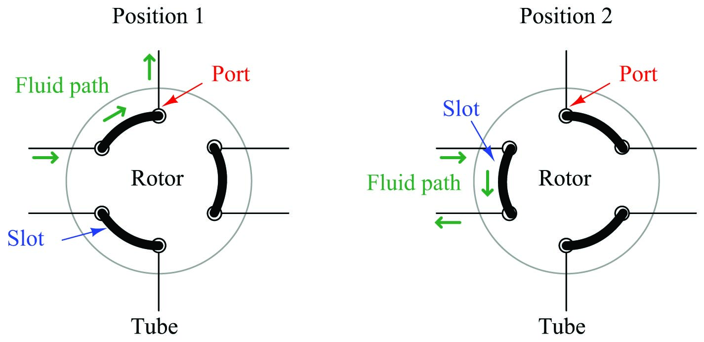
Three slots connect three pairs of ports together. When the rotary valve actuates, the port connections switch, redirecting gas flows.
Connected to a sample stream, carrier stream, and column, the rotary sample valve operates in two different modes. The first mode is a “loading” position where the sample stream flows through a short length of tubing (called a sample loop) and exits to a waste discharge port, while the carrier gas flows through the column to wash the last sample through. The second mode is a “sampling” position where the volume of sample gas held in the sample loop tubing gets injected into the column by a flow of carrier gas behind it:

The purpose of the sample loop tube is to act as a holding reservoir for a fixed volume of sample gas. When the sample valve switches to the sample position, the carrier gas will flush the contents of the sample loop toward the column. This valve configuration guarantees that the injected sample volume cannot vary even if the sample valve’s actuation is not precise. The sample valve need only remain in the “sampling” position long enough to completely flush the sample loop tube, and the proper volume of injected sample gas is guaranteed. An analogy for the sample loop is that of a measuring cup held underneath a continuously-spilling stream of water: so long as the cup is held beneath the stream long enough to completely fill, it is guaranteed to deliver a fixed volume of water when removed from the stream and emptied. Over-filling the cup cannot result in an excessive sample size. Like a measuring cup, the sample loop need only be filled completely with sample gas to deliver a fixed and unerring volume of gas to the chromatograph column when switched from the “loading” position to the “sampling” position.
While in the loading position, the stream of gas sampled from the process continuously fills the sample loop and then exits to a waste port. This may seem wasteful but in fact is quite essential for practical sampling operation. The volume of process gas injected into the chromatograph column during each cycle is so small (typically measured in units of microliters!) that a continuous flow of sample gas to waste is necessary to purge the impulse line connecting the analyzer to the process and thereby ensure a fresh sample, which in turn is necessary for the analyzer to obtain analyses of current conditions. If it were not for the continuous flow of sample to waste, it would take a very long time for a sample of process gas to make its way through the long impulse tube to the analyzer to be sampled, resulting in grossly delayed measurements of process conditions!

Improving chromatograph analysis time
The “Achilles heel” of chromatography is the extraordinary length of time required to perform analyses, compared with many other analytical methods. Cycle times measured in the range of minutes are not uncommon for chromatographs, even continuous “on-line” chromatographs used in industrial process control loops! It is the basic principle of chromatography to separate chemical species using time, and so a certain amount of measurement dead time is inevitable. However, dead time in any measuring instrument is an undesirable quality. Dead time in a feedback control loop is especially bad because enough of it will cause the loop to self-oscillate.
One way to reduce the dead time of a chromatograph is to alter some of its operating parameters during the analysis cycle in such a way that it speeds up the progress of the mobile phase during periods of time where slowness of elution is not as important for fine separation of species. The flow rate of the mobile phase may be altered, the temperature of the column may be ramped up or down, and even different columns may be switched into the mobile phase stream. In chromatography, we refer to this on-line alteration of parameters as programming.
Temperature programming is an especially popular feature of process gas chromatographs, due to the direct effect temperature has on the viscosity of a flowing gas. Carefully altering the operating temperature of a GC column while a sample washes through it is an excellent way to optimize the separation and time delay properties of a column, effectively realizing the high separation properties of a long column with the reduced dead time of a much shorter column:

Another way to speed up the analysis time of a chromatograph is to design it with multiple columns and multiple switching valves, timing the valves so that only the fastest species travel through all columns, while slower species bypass later column stages to exit through the detector first. The alternative is to force all species to elute through all columns (or one long column), which means the minimum cycle time will be determined by the slowest species present in the sample. To use the marathon analogy again, it’s like having to wait until the very last runner crosses the finish line before we can start another race to challenge faster runners. If, however, we stop the race mid-way to shuttle slow runners to the finish line (because we already know they are slow and will never win the race), we can still let the fastest runners compete the entire distance to determine who among them are the fastest, and thereby end the race sooner so we can move on to the next race:

A sequence for one type of dual-column gas chromatograph begins with the sample valve injecting a precise quantity of sample into the first column. In this illustration, the sample is comprised of 6 species labeled 1 through 6 in the order of their elution speed through the columns:

In the next step, the six species elute through column 1, with species 1 through 3 making it into the second column while species 4 through 6 are still working their way through column 1:
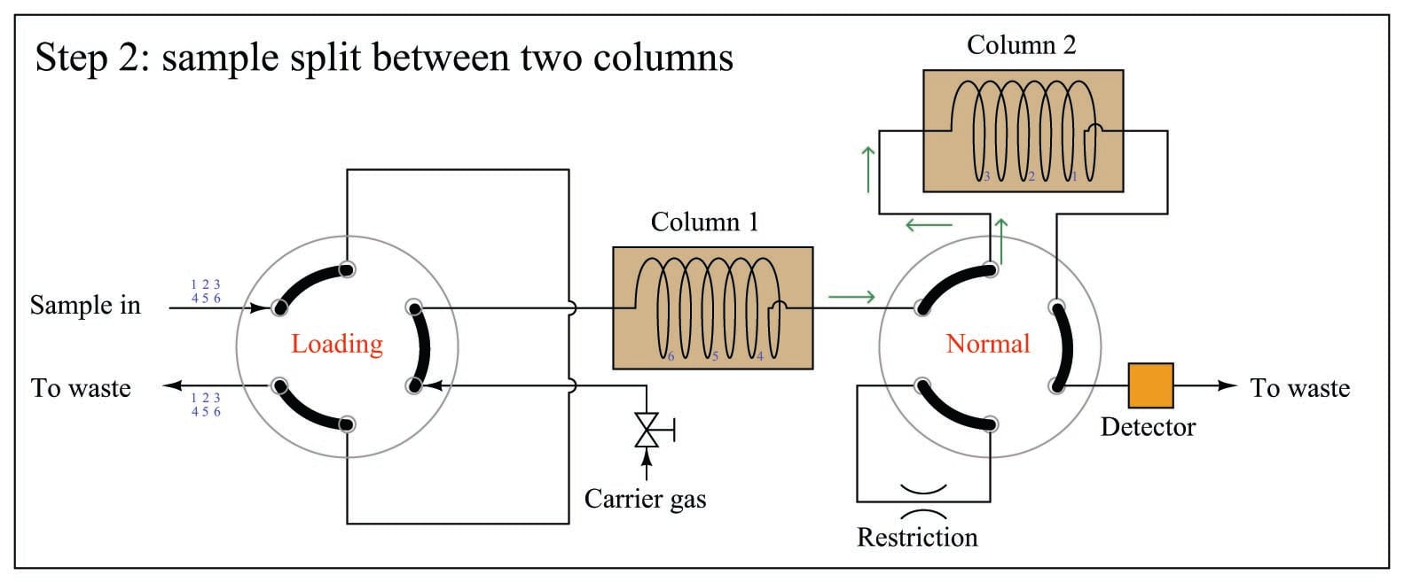
At this point in time, the dual-column valve switches into bypass mode, trapping the faster species (1 through 3) inside of column 2 while allowing the slower species (4 through 6) time to exit column 1 and pass through the detector:

In the last step, the dual-column valve switches back to its normal mode, allowing species 1 through 3 to elute through column 2 and pass through the detector:

The dual-column valve’s timed switching from normal to bypass and back to normal again permits the slowest species to skip past the second column, while the fastest species must elute through both columns for maximum separation. This dual-column switching greatly reduces the total retention time of the sample without sacrificing separation of the fastest species.
A few noteworthy points must be raised with regard to multi-column chromatographs. First, the example shown in the preceding diagrams is not the only type of multi-column chromatograph. “Trapping” a series of sample compounds inside a column is not the only way to provide different compounds with different column paths for faster separation. Some multi-column chromatographs, for example, use “backflush” valves to reverse flow through one or more columns in an effort to avoid having the slowest species elute through the entire length of those columns. This technique is used in applications where separation among compounds in the “slow” group is not important, since backflushing tends to reverse any separation that took place in the column previously.
The next point regarding multi-column chromatographs is that the dual-column valve timing must be precisely set according to known retention times of the different species inside the different columns. In the example GC shown previously, this means the retention times of the transition species (3 and 4 in this case) through the first column must be precisely known, so the dual-column valve may be switched into bypass mode after species 3 exits the first column but before species 4 exits the first column. The retention time of the slowest species (6) must also be precisely known so that the dual-column valve will not switch back to normal mode too soon and route any of that species into the second column where it would take much more time to leave the system.
A final point regarding multi-column chromatographs is that the order of species progression through the detector will not be fastest to slowest as with single-column chromatographs. In the dual-column GC shown previously, the slower group will exit first in order of speed (4, 5, 6), then the fastest group will exit last in order of speed (1, 2, 3).
