Facebook
 Google
 GitHub
 Linkedin
An Introduction to Key Algorithms Used in SLAM
The use of algorithms is essential in order to get simultaneous localization and mapping (SLAM) to work successfully. This article introduces some of the main algorithms used, both common and state-of-the-art.
SLAM, as discussed in the introduction to SLAM article, is a very challenging and highly researched problem. Thus, there are umpteen algorithms and techniques for each individual part of the problem. SLAM needs high mathematical performance, efficient resource (time and memory) management, and accurate software processing of all constituent sub-systems to successfully navigate a robot through unexplored environments.
This article explains the different common and state-of-the-art algorithms for localization, mapping, sensor information processing, data association, feature detection, data filtering, and other miscellaneous processes involved in SLAM. Before diving into SLAM’s algorithms, it is recommended to learn more about the importance of mapping and localization.
How Are Algorithms Used in SLAM?
SLAM is a blanket term for multiple algorithms that pass data from one processing to another. The concept of SLAM itself is modular, which allows for replacement and changes in the pipeline. Thus, very often, several algorithms are developed and used in tandem or compared to converge the best one.
The stochastic nature of the involved algorithms in SLAM and the lack of repeatability in performance renders SLAM unacceptable for deployment in uncontrolled critical environments. Due to the extent of uncertainties and vividness in the environment, SLAM algorithms are difficult to work across all operational environments. For example, SLAM implementation successful in a warehouse may not be as efficient in a shopping mall without human intervention.
Robot Localization Algorithms
The robot pose is a vector and thus can be defined in different reference frames. Measurements from cameras and rangefinders are converted from their local reference frame to the robot frame for localization. Absolute robot pose and absolute landmark positions are determined with respect to a common global reference frame.
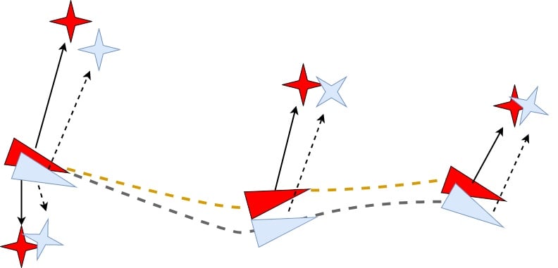
Figure 1. Localization using landmarks. Red = Actual, Blue = Probabilistic
Localization algorithms use multiple sensors, data association, and correction techniques to determine the most accurate robot pose. The individual algorithms and techniques for robot localization include:
- Odometry Estimation
- The motor encoders and wheel dimensions are used to find wheel rotations and use forward kinematics of the mobile robot to compute the current pose. This technique is prone to inaccuracies due to wheel slips and erroneous hardware models, which deteriorate readings over time.
- The onboard IMU readings are integrated at each timestep to compute the robot pose. Measurements from individual sensors in the IMU are fused, often using Kalman filters to avoid drift or bias, but are still not terribly stable.
- Using the onboard camera, visual odometry estimation techniques map the change in the location of feature pixels in 3D images to corresponding frame transformations for the robot pose. This involves methods for feature detection, data association, deep learning, and optical flow.
- Exteroception
- When rangefinders detect the landmarks using data association and feature detection techniques, they are able to determine the change in the positions of the previously detected landmarks and map it to the corresponding change in robot pose that causes it.
- RFID tags, QR-codes, and other marker-based localization techniques are also used, but are limited in application to structured and mapped environments.
Localization is a recursive exercise done at each timestep to either determine the current pose or make corrections to the previous sequence of poses. This is because, as the map evolves and becomes more accurate over time with more exploration and more sensing, the errors in the previous poses are corrected which in turn helps enhance the map.
Common probabilistic techniques used in the industry are Markov Localization, Kalman Localization, and Monte Carlo Localization.
Markov Localization Algorithm
The Markov Localization algorithm starts with an arbitrary probability distribution for the robot's existence in each discrete pose and updates it over time using sensor and odometry information. Keeping track of such large states and individually updating the probabilities is memory- and time-consuming, thus very inefficient.
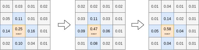
Figure 2. Continuous pose probability updates
Kalman Localization Algorithm
The Kalman Localization algorithm is a more efficient use of the recursive Bayes estimation concept. It models the probability of the robot’s pose as a Gaussian and updates the mean and the variance of the distribution until the values converge to almost constant. The iterative approach uses the motion model and the observation models to estimate and update the belief in each Bayesian loop.
Monte Carlo Localization Algorithm
The Monte Carlo Localization algorithm uses a particle filter approach to recursively determine the robot pose. It is the most efficient of the three and further enhancements in importance sampling and implementation of the particle filter also enhance its performance.
Robot Mapping Algorithms
Generating environment maps and updating them recursively is a computationally expensive step. Defining the appropriate data structure to store the map is vital to system performance.
There are several techniques used to create and update the robot map. The most common ones include:
- Inverse Sensor Model
Given a LiDAR rangefinder and a start occupancy grid, the probability of a grid cell being occupied is computed at each timestep. For each cell, one of the rays of the rangefinder is associated with it.Depending on if the range for that ray ends at the cell or not, it is determined if the cell is blocking the ray or not. Further details of the implementation are outside the scope of this article but can be explored here. This is a very time-consuming step as it loops over all individual cells.
- Ray Tracing
Ray tracing loops over each ray of the rangefinder and updates the occupancy grid cells along the ray. Thus, it saves computational resources and is more efficient.
- Visual Sensing
Visual sensing obtains different high-definition maps of the environment, usually 3D, and detects features and patterns to populate occupancy grids or feature maps. It also detects surfaces and contours using 3D point clouds.
- Maximum-Likelihood
The maximum-likelihood incremental technique uses the previous map, current robot pose, and current nearby sensing to update the current map. While it is not probabilistic and hence avoids stochasticity, it is slow due to large processing needs.
Algorithms for Exteroceptive Sensors
Random Sampling and Consensus (RANSAC) is used for feature extraction, like edge detection using rangefinder readings, iteratively. It uses the information from rangefinders (an array of tuples of distance and bearing) coming through to create lines and consequently derive landmarks.
Iterative Closest Point is used on point cloud information for localization and data association purposes.
Optical flow is generated using algorithms like Lucas-Kanade on input images from onboard cameras to eventually derive corresponding geometric transformations and motion of the robot.
Motion Planning Algorithms
Once the environment is mapped, the robot is capable of autonomous navigation while avoiding dynamic obstacles. When the robot is instructed to travel from one point to another, the motion planning algorithm defines the pipeline for finding a path for the motion and the ideal motion profile for the robot.
Usually, hierarchical planners are implemented in such motion planning tasks. The pipeline uses global planners for high-level planning over the predefined static maps and local planners for dynamic intermediate path planning along the path proposed by the former.
Common global planning algorithms include search-based planners like A*, Djikstra, and several other variants as well as sampling-based planners like RRT, PRM, and their variants. Local planners used in industry and academia alike include the trajectory rollout algorithm, dynamic windowing algorithm, and timed-elastic band planner.
Miscellaneous Algorithms
- Kalman filter and Extended Kalman filter are used for sensor fusion for linear and non-linear systems respectively.
- Particle filter is a non-parametric version of the localization filters that uses multiple particle hypothesis for state estimation
- SIFT, SURF, ORB, and BRIEF are several algorithms for image feature extraction in visual SLAM applications.
- Deep-learning-based object detection, tracking, and recognition algorithms are used to determine the presence of obstacles, monitor their motion for potential collision prediction/avoidance, and obstacle classification respectively.
- Collision detection in dynamic environments is done by preempting motion and running collision checks for the robot footprint against potential 2D area overlap with elements in the scene.
- Motion prediction for different objects in the scene obtained object classification helps in avoid or preempt collisions.
Existing Software Solutions for SLAM
SLAM has been a research problem in the robotics industry and academia for decades. There are a few ready-to-use packages and libraries for SLAM or sub-problems of SLAM:
- Gmapping - Complete SLAM package (ROS Implementation)
- AMCL - Adaptive Monte Carlo Localization package for laser scanner-based 2D localization
- Robot_pose_ekf - ROS package to combine data from IMU, computer vision, and laser scanners for 3D robot pose estimation
- Rtabmap - Real-time Appearance-based mapping package for SLAM (ROS Implementation)
- ORBSLAM - Vision-based SLAM package for monocular, RGB-D, and stereo cameras
- Octomap - A library for 3D occupancy grids
Just the Beginning of Algorithms Used in SLAM
Many of the algorithms discussed in the article are used in the off-the-shelf libraries and software packages mentioned above. While this list is not exhaustive due to the sheer nature of how intangible SLAM research and development is today, this article covers the most common, robust, and successful (across substantial scenarios) algorithms deployed.
To conclude, SLAM is highly dependent on Kalman filters and sensors. This ends the introductory series of articles on SLAM and encourages users to explore the different aspects of SLAM.