Robot Manipulation Control with Inverse and Forward Kinematics

What is the Kinematic Chain? 

Donald L. Pieper invented the 321 kinematic chain. It is used in most robotic arms with high Degrees of Freedom (DoF) and is made of intersecting revolute joints. 

The Stanford arm was one of the first models of this design. It had six degrees of freedom from two revolute joints, a prismatic joint and a spherical joint. Most robotic arms used in industry are advanced iterations of the Stanford arm. 

 

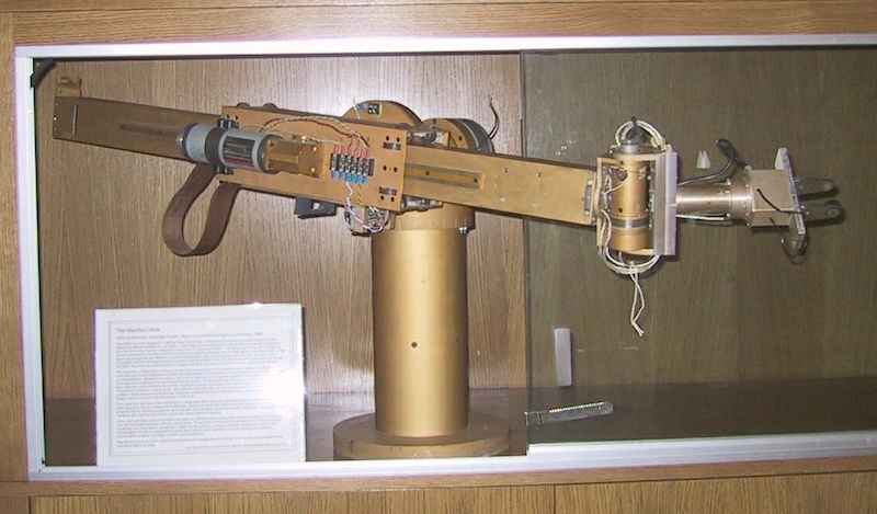
The Stanford arm. Image used courtesy of Stanford University

 

An engineer can use forward kinematics and inverse kinematics to figure out the positions of end effectors and manipulate the robotic arm.

 

Forward Kinematics

In any kinematic chain, from the base of the robotic arm, different links are serially connected with revolute links or prismatic joints. The end effector or tooltip is attached at the end of the last link. Forward kinematics can calculate the position and orientation of the end effector with joint variables.

 

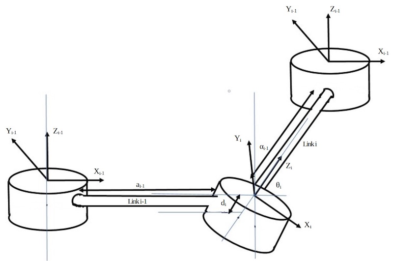
Figure 1: Representative image of kinematic chain showing Denavit Hartenberg parameters and reference frames. Information used courtesy of S. Kucuk and Z. Bingul

 

The Denavit-Hartenberg method is the commonly used method for the forward kinematics model. It uses four parameters at each axis to define a system. They are:

• a_i-1 representing the link length
• α_i-1 denotes the link twist
• d_i stands for link offset
• θ_i for the joint angle

 

Denavit-Hartenberg’s model is used when there are multiple reference frames in a system. Different reference frames can be placed at each joint. Z_i is pointing in the direction of rotation at the joints or the direction in which the joint slides to and from. Denavit-Hartenberg parameters are decided after the axes of coordinate frames are determined at each joint.

Suppose coordinate frames and DH parameters are clearly marked. The link length a_i-1 is measured as the length between the axes Z_i and Z_i-1 along the X_i-1 axis. α_i-1 is the angle between the same two Z axes measured along the X_i axis.

d_i is the distance between X_i-1 and X_i measured along the Z_i axis, and θ_i is the angle between X_i-1 and X_i. The general Transformation matrix T^_ii-1 for a link can be written as follows.

 

T^_ii-1=R_x(a_i-1) D_x(a_i-1)R_z(θ_i)Q_i(d_i)

 

Similarly, the transformation matrix for the reference frames at each joint can be calculated, TT⁰₁, T¹₂,... The transformation matrix of the end effector in relation to the base can be calculated by multiplying the transformation matrix at each joint.

 

T^base_end-effector =  T⁰₁T¹_2...T^n-1_n

This transformation matrix will give p_x, p_y, and p_z, the position coordinates of the end-effector.

 

Inverse Kinematics

Calculating the position of the end-effector with forward kinematics is not sufficient for controlling robotic arms. We need to calculate how to reach the desired state of the arm from the current state by reconfiguring the kinematic links. The calculations for it are referred to as inverse kinematics.

Inverse kinematics can be solved using the geometric solution approach or the algebraic solution approach. Let's take a brief look at the two approaches.

 

Geometric Solution Approach

In this method, the joint space is divided into multiple two-dimensional planes and trigonometrically finding solutions in each plane.

 

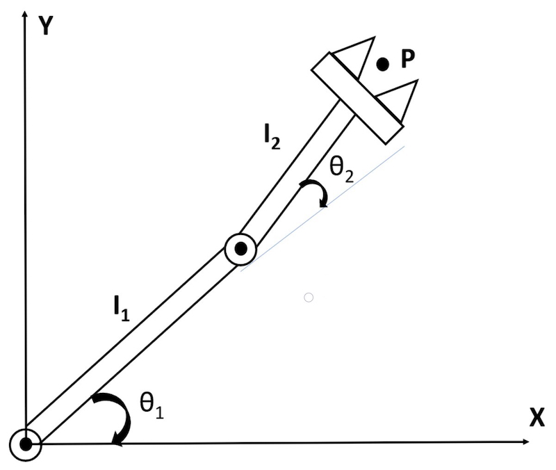
Figure 2: For example, consider a manipulator with two degrees of freedom. Information used courtesy of S. Kucuk and Z. Bingul

 

This can be simplified to a simple geometric problem, as shown below.

 

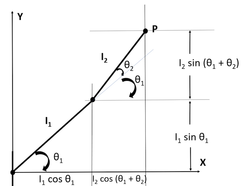
Figure 3: Now, simple geometry can be applied to calculate the parameters. Information used courtesy of S. Kucuk and Z. Bingul

 

However, it gets far too complex and time-consuming to calculate when robotic arms with higher degrees of freedoms are involved. 

In some robotic arms, the manipulator only operates in two dimensions. In other robotic arms, it operates in three-dimensional space. Keeping track of the different two-dimensional planes with respect to each other becomes tedious with a higher number of joints.

 

Algebraic Solution Approach

In forward kinematics, the transformation matrix for the end effector to the base is found by multiplying all the transformation matrices at joints.

 

T^base_end-effector =  T⁰₁T¹_2...T^n-1_n

 

For six-axis robots with six degrees of freedom, the equation becomes:

 

T⁰₆ =T⁰₁T¹₂T²₃T³₄T⁴₅T⁵₆

 

To find the inverse kinematic solution for the first joint, the inverse matrix of the transformation matrix T⁰₁ (which is [T⁰₁]^-1) to both sides of the equation above.

 

[T⁰₁]^-1T⁰₆ = [T⁰₁]^-1T⁰₁T¹₂T²₃T³₄T⁴₅T⁵₆

 

For a robotic arm with six degrees of freedom, 12 algebraic equations need to be solved to get the joint space parameters of one joint. Similarly, the joint space parameters for all six joints can be found. 

It takes a long time to solve it manually. Today with access to advancing computing power, algorithms can solve it in a fraction of a second. This makes it simpler than the geometric solution approach in modern-day applications.

For a kinematic chain, forward kinematics is to calculate the end-effector position in relation to the base. The Denavit-Hartenberg parameters are used for mathematical calculations as it has variables to represent rotational and translational parameters.

The transformation matrix for each joint can be individually calculated and multiplied to obtain the T^end-effector_base. This final matrix gives the position coordinates of the end effector.

 

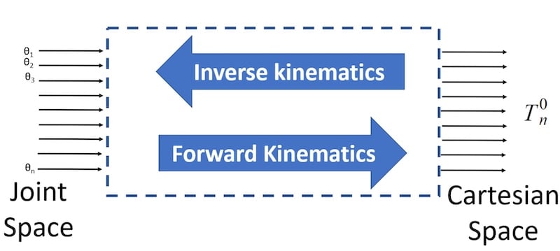
Figure 4: Inverse kinematics is used to find the joint space parameters when Cartesian parameters are known. This is essential to manipulate the end effect by inducing different movements to the different joints.

 

In simple terms, forward kinematics is used to convert variables in joint space (Denavit-Hartenberg parameters) to Cartesian coordinates, and inverse kinematics is used for the reverse operation.
Using these kinematic methods can help engineers understand how to control robot arms more carefully.