Understanding the Derivative Term in PID Control

Hot opinion: calculus class would be a lot more fun if they brought motors into the classroom. I didn’t understand any practical applications of integrals and derivatives until learning about feedback in motion controls. Proportional and integral controls are relatively easy to understand (and they have been demonstrated previously), but the derivative term can be a bit more tricky to visualize in a real system.

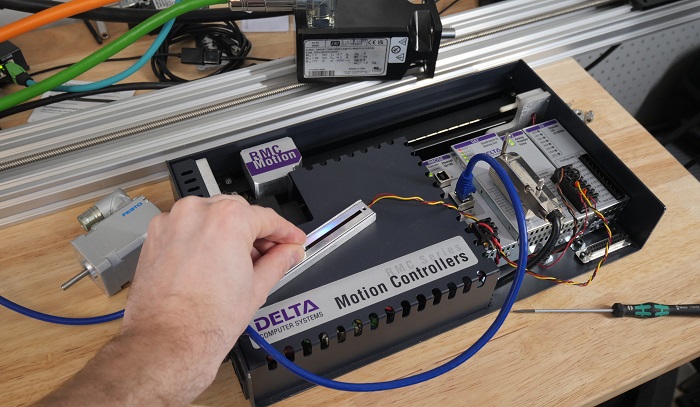
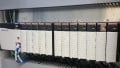
Figure 1. This trainer uses a linear potentiometer as a set point signal so that it can be changed quickly but not instantly, which is useful for our demonstration.

Thanks to the Delta Motion team in Battle Ground, WA, I was able to borrow a training unit that can help us visualize these PID gains like never before.

What is a Derivative?

There is no sense in explaining the result of an equation if we don’t understand the term in the first place.

A derivative is a mathematical model that allows us to look at how fast something is moving or changing at a single, specific point in time. Formally, they call this a ‘rate of change’ of a variable with respect to time.

A physical example is a car in motion. As you are driving, you change location every moment. However, you’re probably speeding up and slowing down all the time, depending on traffic and stop lights. This means that, while you may have driven 10 miles in 20 minutes, your speed at any moment could be fast or slow. The derivative is not an average velocity, but an instantaneous value where the elapsed time is virtually zero. It gives us a close look at what is happening right NOW.

Figure 2. In the car example, the physical ‘rate of change’ is velocity. But in motion control, the derivative turns the instantaneous error into the ‘rate of change’ of the error.

How Does This Relate to Motion Control?

When objects are in motion, they want to remain in motion, based on Newton’s laws. If we are coming up to a target very quickly, we should slow down or we might overshoot. On the other hand, if the target is getting further away from us, we should increase the control output to remain accurately on target.

Output control is based on the ‘error’ measured by the system, which is the difference between the set point and the current value. This error is constantly being evaluated, and the controller can determine a few things about the error. What is the error right now (Kp)? How much is the error adding up over time (Ki)? And how fast is the error changing?

For each of these questions, we have a PID term. How fast is the error changing? That’s the job for our new term Kd, or derivative control.

It’s taken us a while to get through the definitions, so let’s look at a couple of examples. First, we should examine a motion profile that does not include any derivative gain; a PI-only controller. Both values are low, so that you can clearly see the combined effect.

Figure 3. A slow-response system with P and I gains, but no D gain. This plot is used to establish a baseline reference for the next visual.

Low D Gain

When a low derivative gain is applied, the effects are most visible while the set point is changing somewhat abruptly. When the set point changes faster than the system can respond, the error will grow large for a moment; its rate of change will be high.

In response, the output control will also be higher for a brief moment when the set point potentiometer is being adjusted. You can see this as a steeper slope in the current value curve (red line), which suddenly decreases back to a normal curve right when the input stops changing, since now, the error is decreasing.

Figure 4. A system response with low D gain. The system responds quickly as the set point is changed, then more slowly when the set point becomes constant.

To explain further, when the set point stops changing and the system is catching up, the difference between the set point and the current value (error) gets smaller and smaller. In this case, the rate of change is lower, and the output signal will also decrease. Since the influence of the Kp and Ki terms causes the output to level out as the set point is reached, the compounding influence of Kd will be smaller over time.

High D Gain

When any real system responds with some legitimate Kp and Ki, there is likely to be just a bit of overshoot. One moment, the current value is sitting right on the set point, but the next moment, it’s gone just a bit beyond. In other words, the error went from zero to some new value very, very quickly, and the corresponding rate of change is very high. A high Kd will see this high rate of change and immediately set a high reverse output control signal, and the output will blow right past the set point in the other direction.

What would this mean physically? A very loud ringing, buzzing, horrible vibration and shaking of the equipment as it violently rocks back and forth. I do not have a video of this effect since it was very uncomfortable to watch, even momentarily, although I did experience it with the trainer (my sincerest apologies to the Delta Motion team, but the trainer is just fine).

Derivative gain is a very helpful way to stay on track, but if it’s too high, it can damage the equipment.

What is the Correct Gain Value?

In PID controls, there is no single formula for all systems. The mass, speed, and load of the system, along with many other variables, influence the gain. Think of vehicles: they all contain springs and shock absorbers, but the size and value of each are vastly different depending on the size and purpose of the vehicle.

Tuning is the entire process of analyzing, testing, and optimizing each system to select the correct values, and there are tools to accomplish this task. It can be intimidating, and risky if high-value equipment is in use, but it pays great dividends to understand how physics and software come together to create the best motion solutions.