PID Visualized: Watch Proportional, Integral, and Derivative in Motion

Back in engineering school, I wish I had learned calculus more thoroughly. I think I understood the calculations and how to get (many of) the right answers, but I didn’t really grasp how the terms would be put to use in future life. I could figure out the surface area of a shape between two graphs or the rate of change of a filling tank, but it wasn't until I worked with motion control systems that I actually learned how these algorithms shape automation.

Recently, thanks to the use of a controller and axis from Delta Motion in Battle Ground, WA, I was able to record the input and output waveforms of a graph while the system was live in motion. Being able to adjust the P, I, and D parameters on the fly helps to visualize the impact of each term.

 

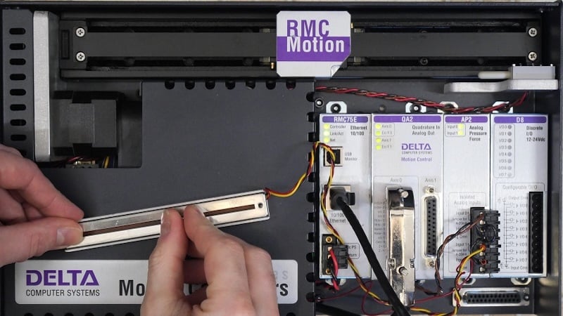
Figure 1. Using motion control can help explain the details of PID gains in a closed-loop system.

 

In this tutorial, we’ll stick to only the P and I terms since nearly all process and motion controls include these, including some dedicated PI controllers. We’ll look at the effects of the D term later.

 

Proportional Gain

As we have seen before in previous articles, a proportional effect is simply when the value of the input variable impacts the output with a constant linear multiplier relationship. If the input is 5 and the gain is 2, then the output will be 10.

Now, putting this into motion terms, the input variable is error, which is the subtraction of the (target position - the current position). The further away from the target position, the larger the error.

Note: In the following discussion, large and small are relative values. In various PID systems, 1 may be a large value, while in others, 500 may be considered small. However, the concept will remain the same, regardless of the magnitude of the final tuned system.

 

Zero Proportional Gain

If we have a zero proportional gain (0.0), the output will be zero, and the motion system will slowly drift off on its own if it moves at all. Any semi-correct response would only be due to an open-loop output command called feedforward. Essentially, no feedback means the system has no idea what it’s doing.

 

Small Proportional Gain

If we add just a little bit of proportional gain (5.0), the system is now able to respond, but still slowly. If we give a position command, the system will begin moving somewhat quickly, but it will slow down long before it reaches the target. In fact, it may become so slow that it stops altogether before reaching the intended target position; we call this a settling error.

 

 

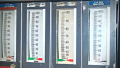
In the videos, we can see three lines on the graph. The blue line is the commanded position, the red line is the actual current position of the actuator, and the final green line is the analog output sent to the controller.

 

Large Proportional Gain

Now, we’ll increase the proportional gain to a larger value (50.0). In this small system with no load, it actually behaves quite well with this gain value. It responds quickly and settles right on the target position, but we can still see a bit of a problem. In some of the larger motions, it tends to overshoot the position and go too far. Without enough output to swing back in the other direction, it will still land a bit off from the intended target.

 

 

Integral Gain

To correct that overshoot and settling error, we need to figure out a way to know if the system has stopped moving but we didn’t make it to the exact target position. Over time, each time the sensor position is recorded, we add any error to an ever-growing cumulative error value. If this keeps growing, it means we’re not far enough. If it begins growing in the negative direction, we have gone too far. If it’s not growing at all, we’re right on target.

The constant accumulation of individual values over a period of time is exactly what an integral does—the integral of error over time. The accumulated error, multiplied by the integral gain, will get the system moving again, just a bit if we lose speed due to the proportional-only control.

Since this is a low-inertia system, we’ll test the following parameters with a low proportional gain installed just to be able to see the effects.

 

Small Integral Gain

If the integral is small (0.75), the motion curve looks like a proportional-only control right at first. But as time goes by, we can see the current value creeping closer to the target position. It does take a while since the error is accumulating slowly–not exactly a high-speed response.

 

 

Large Integral Gain

If we have some error accumulating, but we multiply it by too large of a gain (100), we will apply too much output too quickly, and the system will go too far. And then it must turn around and go back, likely also overshooting back and forth in quick oscillation. It may look neat on a graph, but we want to find a sweet spot value between small and large.

 

 

A second test is to try a large integral gain (this time, 1000) when we have also installed a large proportional gain (100). This time, there is some initial system overshoot because of the large proportional gain and the added integral gain, giving the system a lot of momentum right as the input command is asserted. However, right after the overshoot, it quickly responds to correct itself with the classic concave slope that is characteristic of integral gain.

 

 

Proper PI Gain

In our last example, we choose a fairly high proportional gain to provide a quick initial reaction (100) and a somewhat low integral gain so that the error is instantly corrected but avoids the problematic overshoot and oscillation (10).

 

 

This final example shows a great response. The blue set point signal is nearly invisible behind the red current position signal, and, for this motion control application, that’s exactly what we want.

 

All videos and images used courtesy of the author