 Facebook
 Google
 GitHub
 Linkedin
P, I, and D Responses Graphed
Visualizing the actions of P, I, and D tuning parameters using graphs is extremely useful in predicting the repose of the system when adjusting individual gain values. |
A very helpful method for understanding the operation of proportional, integral, and derivative control terms is to analyze their respective responses to the same input conditions over time.
PID Controller Tuning Parameters
This section is divided into subsections showing P, I, and D responses for several different input conditions, in the form of graphs. In each graph, the controller is assumed to be direct-acting (i.e. an increase in process variable results in an increase in output).
It should be noted that these graphic illustrations are all qualitative, not quantitative. There is too little information given in each case to plot exact responses. The illustrations of P, I, and D actions focus only on the shapes of the responses, not their exact numerical values.
In order to quantitatively predict the PID controller responses, one would have to know the values of all PID settings, as well as the original starting value of the output before an input change occurred and a time index of when the change(s) occurred.
System Response: Single Step Input
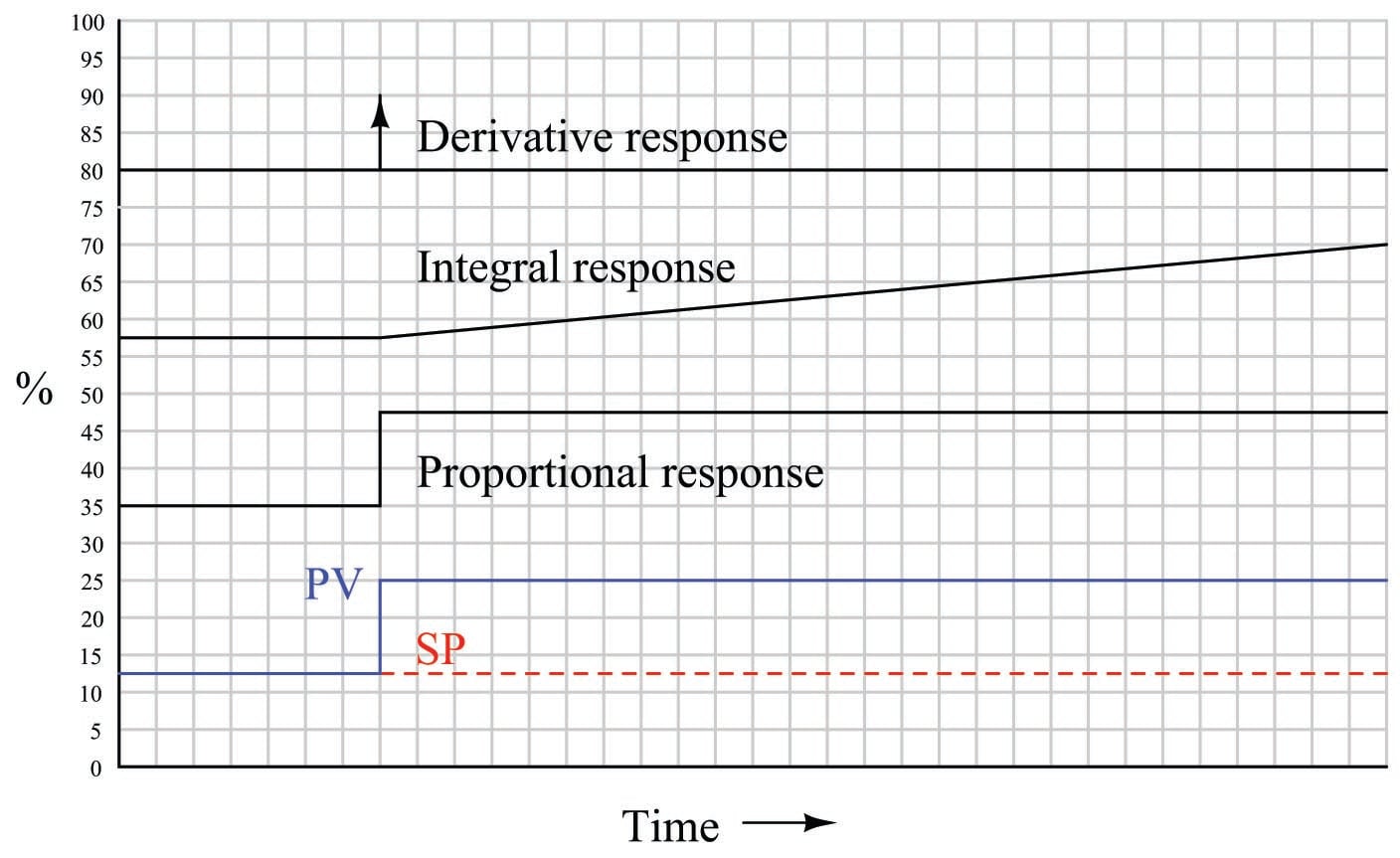
Proportional action directly mimics the shape of the input change (a step). Integral action ramps at a rate proportional to the magnitude of the input step. Since the input step holds a constant value, the integral action ramps at a constant rate (a constant slope). Derivative action interprets the step as an infinite rate of change, and so generates a “spike” driving the output to saturation.
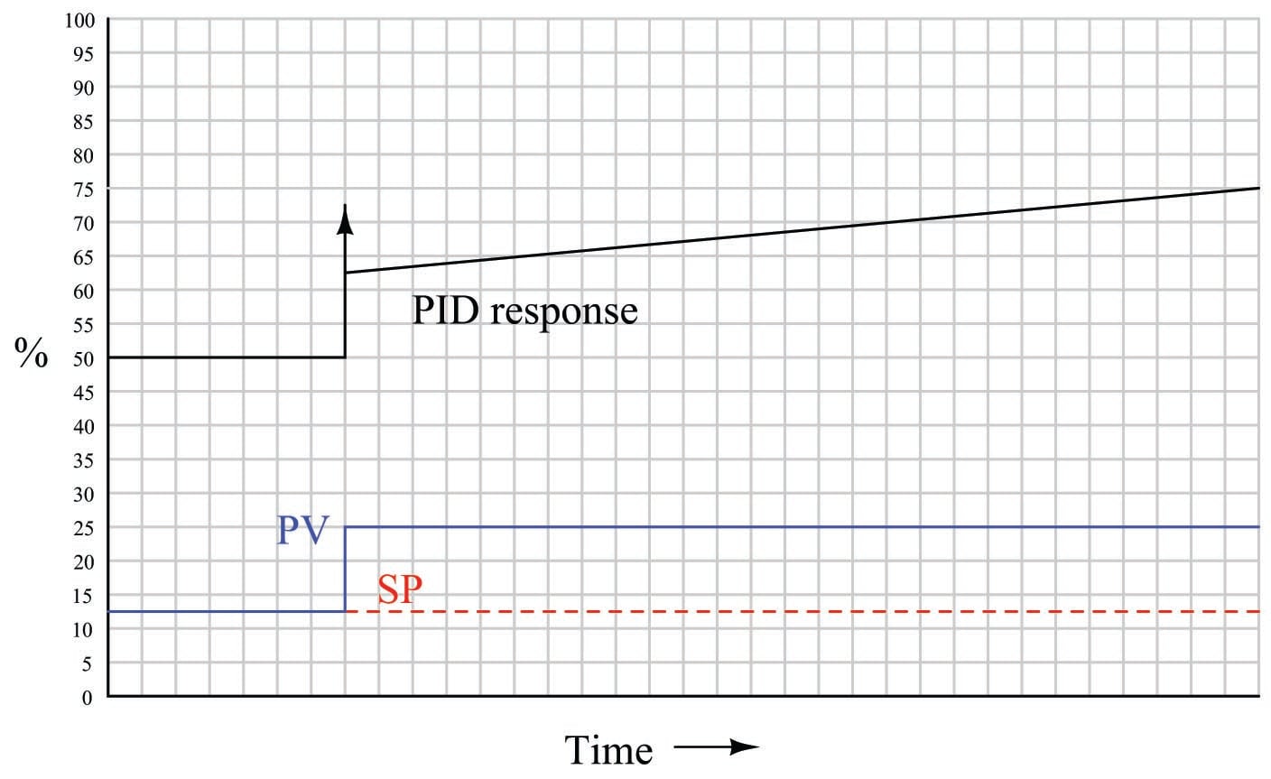
When combined into one PID output, the three actions produce this response:
System Response: Pulse Input Step-and-Return
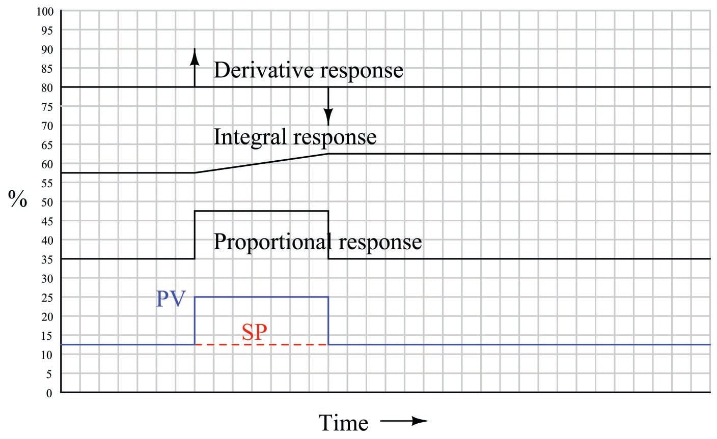
Proportional action directly mimics the shape of the input change (an up-and-down step). Integral action ramps at a rate proportional to the magnitude of the input step, for as long as the PV is unequal to the SP. Once PV = SP again, integral action stops ramping and simply holds the last value. Derivative action interprets both steps as infinite rates of change, and so generates “spikes” at the leading and at the trailing edges of the step. Note how the leading (rising) edge causes derivative action to saturate high, while the trailing (falling) edge causes it to saturate low.
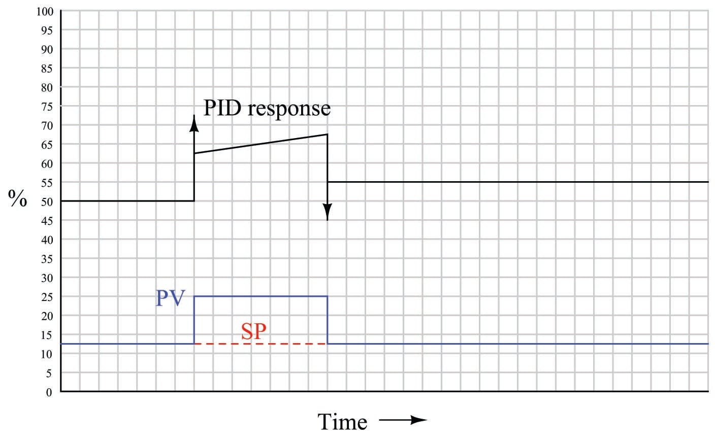
When combined into one PID output, the three actions produce this response:
System Response: Two Bipolar Pulses
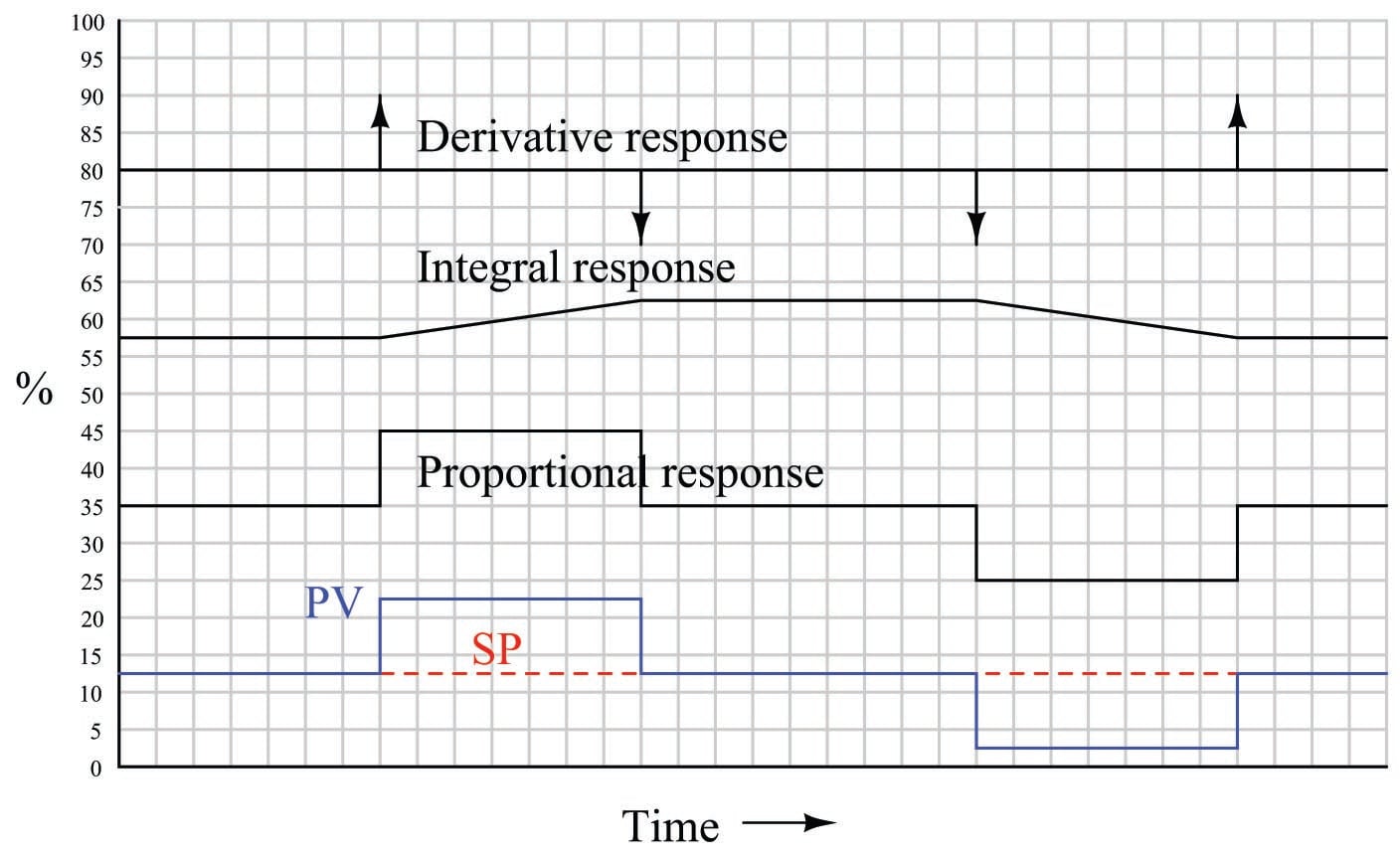
Proportional action directly mimics the shape of all input changes. Integral action ramps at a rate proportional to the magnitude of the input step, for as long as the PV is unequal to the SP. Once PV = SP again, integral action stops ramping and simply holds the last value. Derivative action interprets each step as an infinite rate of change, and so generates a “spike” at the leading and at the trailing edges of each step. Note how a leading (rising) edge causes derivative action to saturate high, while a trailing (falling) edge causes it to saturate low.
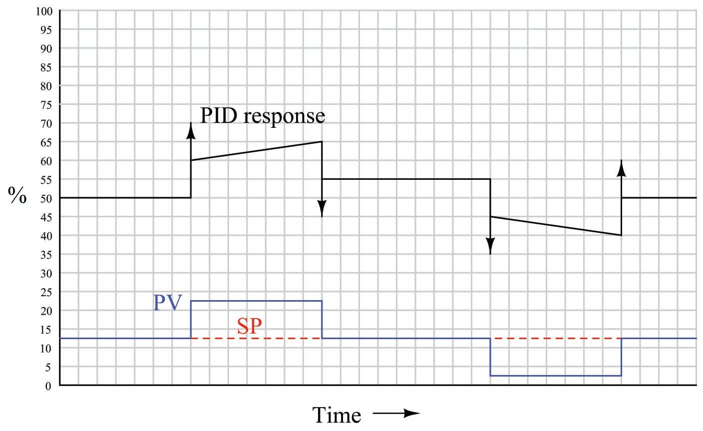
When combined into one PID output, the three actions produce this response:
System Response: Ramp-and-Hold
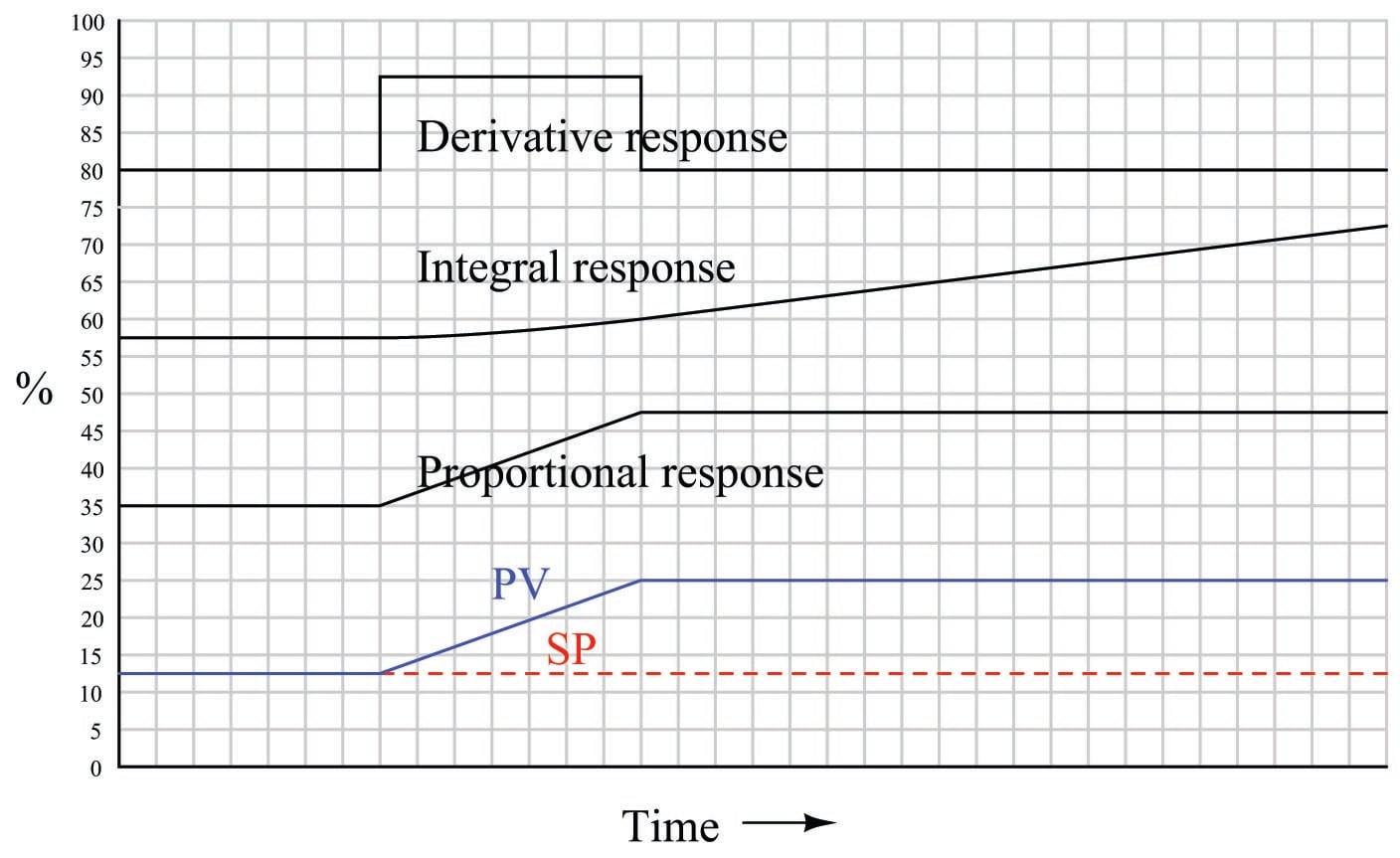
Proportional action directly mimics the ramp-and-hold shape of the input. Integral action ramps slowly at first (when the error is small) but increases ramping rate as error increases. When error stabilizes, integral rate likewise stabilizes. Derivative action offsets the output according to the input’s ramping rate.
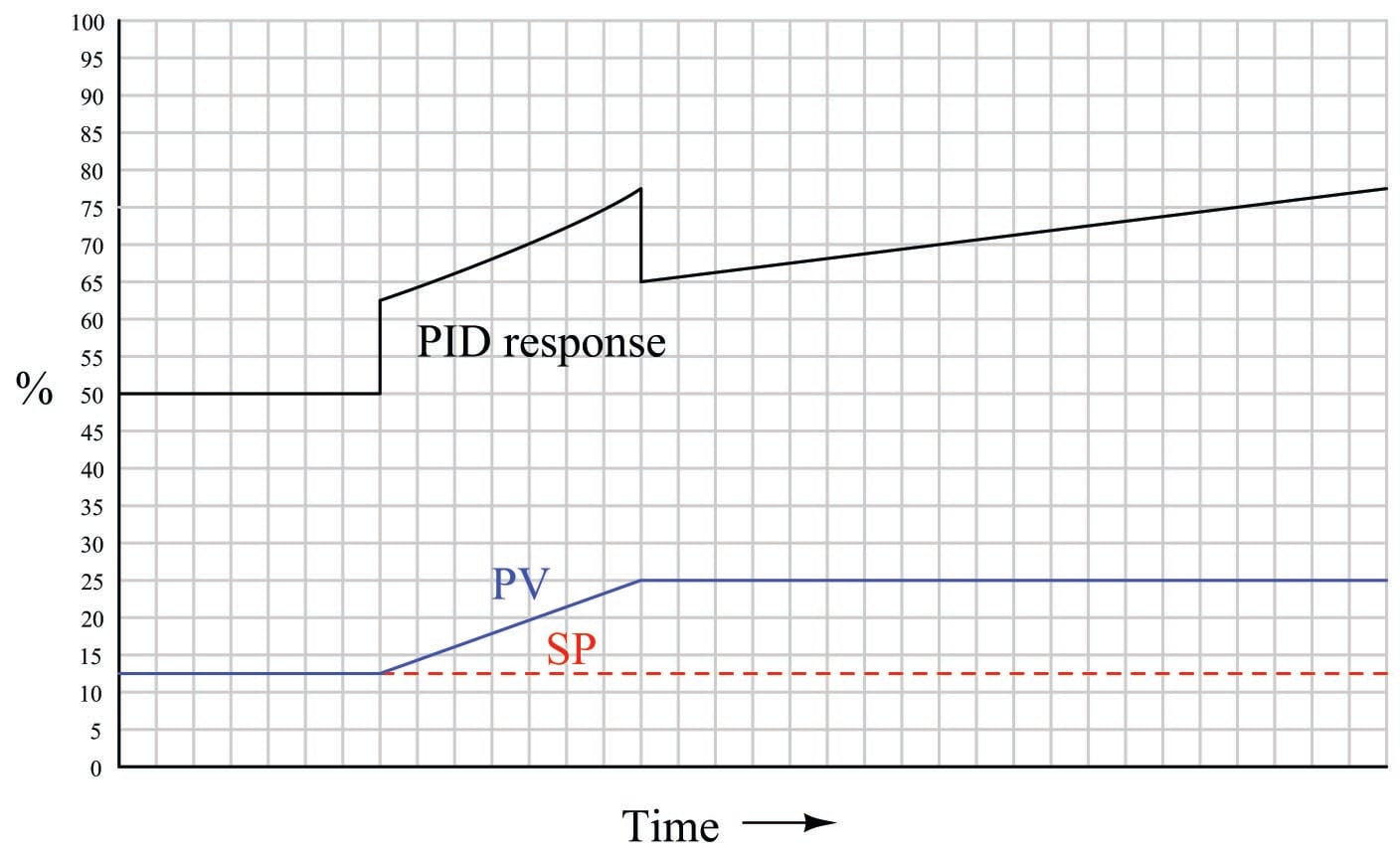
When combined into one PID output, the three actions produce this response:
System Response: Ramp Up and Ramp Down
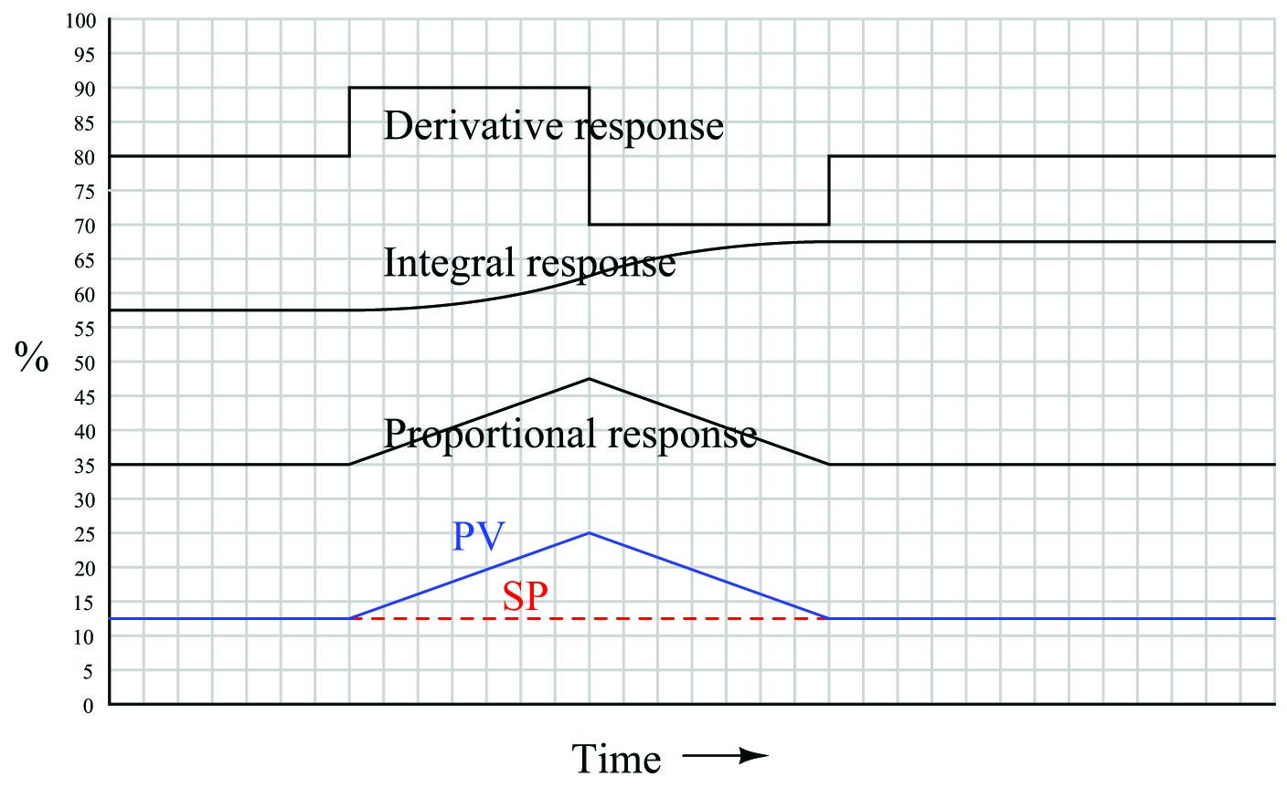
Proportional action directly mimics the up-and-down ramp shape of the input. Integral action ramps slowly at first (when the error is small) but increases ramping rate as error increases, then ramps slower as error decreases back to zero. Once PV = SP again, integral action stops ramping and simply holds the last value. Derivative action offsets the output according to the input’s ramping rate: first positive then negative.
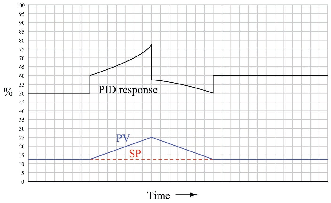
When combined into one PID output, the three actions produce this response:
System Response: Multi-slope Ramp
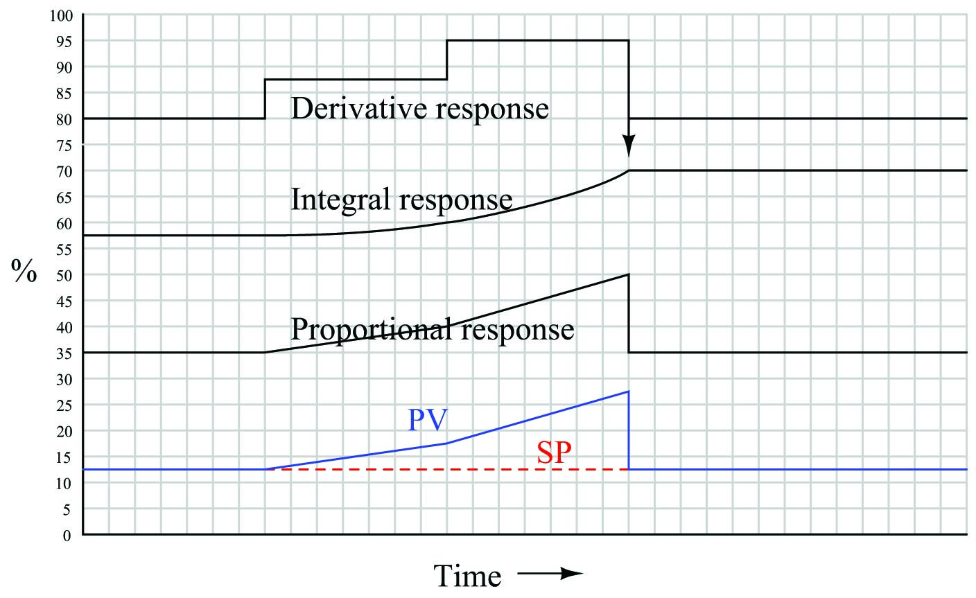
Proportional action directly mimics the ramp shape of the input. Integral action ramps slowly at first (when the error is small) but increases ramping rate as error increases, then accelerates its increase as the PV ramps even steeper. Once PV = SP again, integral action stops ramping and simply holds the last value. Derivative action offsets the output according to the input’s ramping rate: first positive, then more positive, then it spikes negative when the PV suddenly returns to SP.
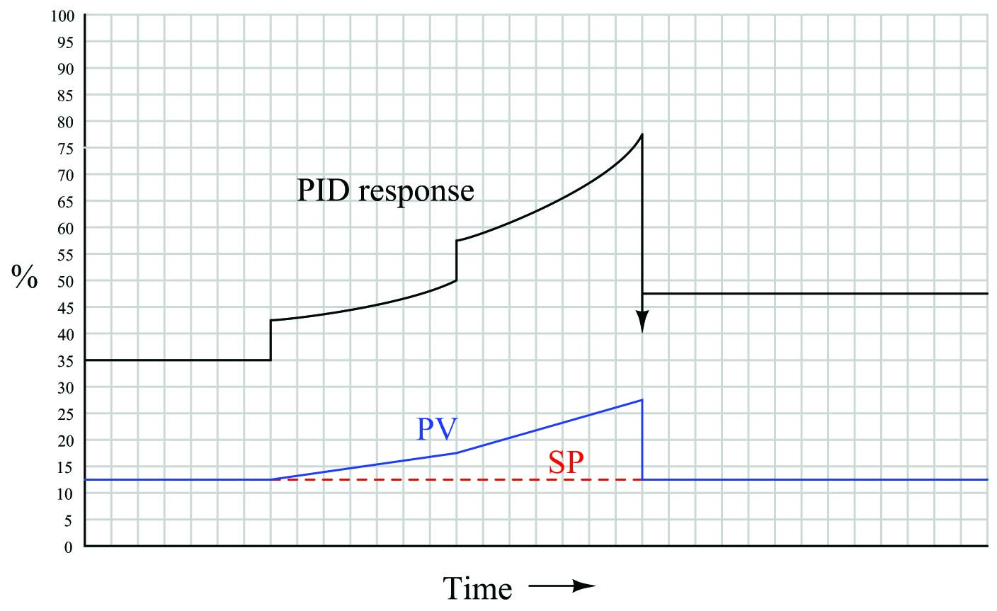
When combined into one PID output, the three actions produce this response:
System Response: Multiple Ramp Steps
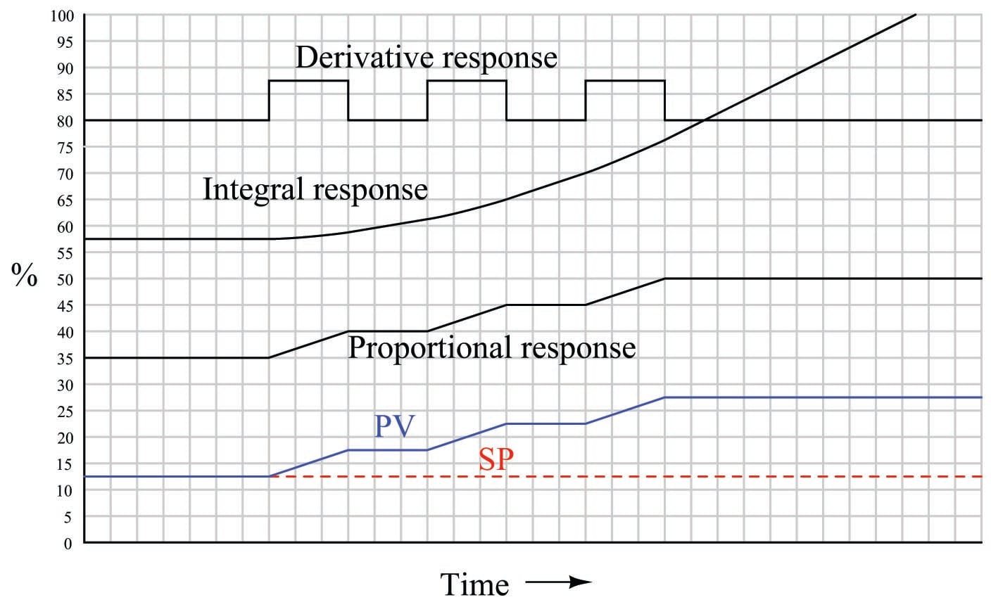
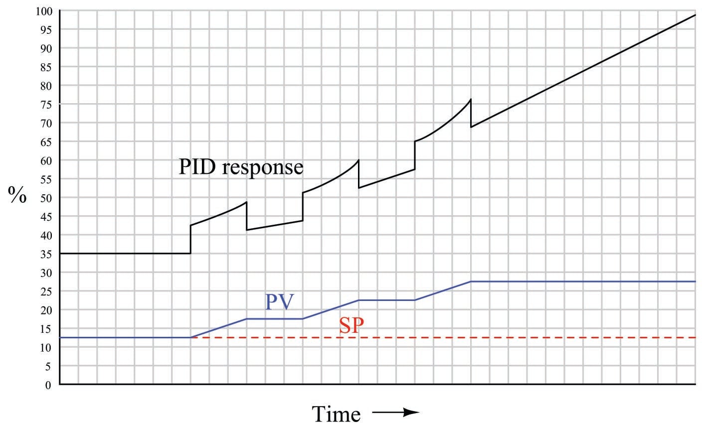
Proportional action directly mimics the ramp-and-step shape of the input. Integral action ramps slowly at first (when the error is small) but increases ramping rate as error increases. Which each higher ramp-and-step in PV, integral action winds up at an ever-increasing rate. Since PV never equals SP again, integral action never stops ramping upward. Derivative action steps with each ramp of the PV.
When combined into one PID output, the three actions produce this response:
System Response: Single Sine Wave
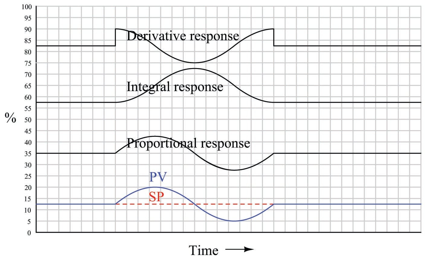
As always, proportional action directly mimics the shape of the input. The 90\(^{o}\) phase shift seen in the integral and derivative responses, compared to the PV wavelet, is no accident or coincidence. The derivative of a sinusoidal function is always a cosine function, which is mathematically identical to a sine function with the angle advanced by 90\(^{o}\):
\[{d \over dx} (\sin x) = \cos x = \sin (x + 90^o)\]
Conversely, the integral of a sine function is always a negative cosine function, which is mathematically identical to a sine function with the angle retarded by 90\(^{o}\):
\[\int \sin x \> dx = - \cos x = \sin (x - 90^o)\]
In summary, the derivative operation always adds a positive (leading) phase shift to a sinusoidal input waveform, while the integral operation always adds a negative (lagging) phase shift to a sinusoidal input waveform.
When combined into one PID output, these particular integral and derivative actions mostly cancel, since they happen to be sinusoidal wavelets of equal amplitude and opposite phase. Thus, the only way that the final (PID) output differs from proportional-only action in this particular case is the “steps” caused by derivative action responding to the input’s sudden rise at the beginning and end of the wavelet:
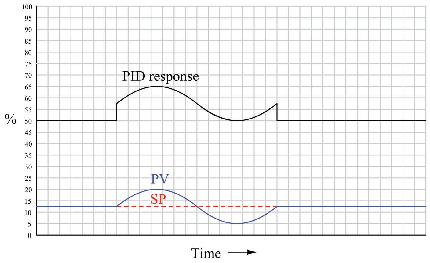
If the I and D tuning parameters were such that the integral and derivative responses were not equal in amplitude, their effects would not completely cancel. Rather, the resultant of P, I, and D actions would be a sine wavelet having a phase shift somewhere between \(-90^{o}\) and \(+90^{o}\) exclusive, depending on the relative strengths of the P, I, and D actions.
The 90 degree phase shifts associated with the integral and derivative operations are useful to understand when tuning PID controllers. If one is familiar with these phase shift relationships, it is relatively easy to analyze the response of a PID controller to a sinusoidal input (such as when a process oscillates following a sudden load or setpoint change) to determine if the controller’s response is dominated by any one of the three actions. This may be helpful in “de-tuning” an over-tuned (overly aggressive) PID controller, if an excess of P, I, or D action may be identified from a phase comparison of PV and output waveforms.
Note: Regarding Quantitative Graphing
A common exercise for students learning the function of PID controllers is to practice graphing a controller’s output given input (PV and SP) conditions, either qualitatively or quantitatively. This can be a frustrating experience for some students, as they struggle to accurately combine the effects of P, I, and/or D responses into a single output trend. Here, I will present a way to ease the pain.
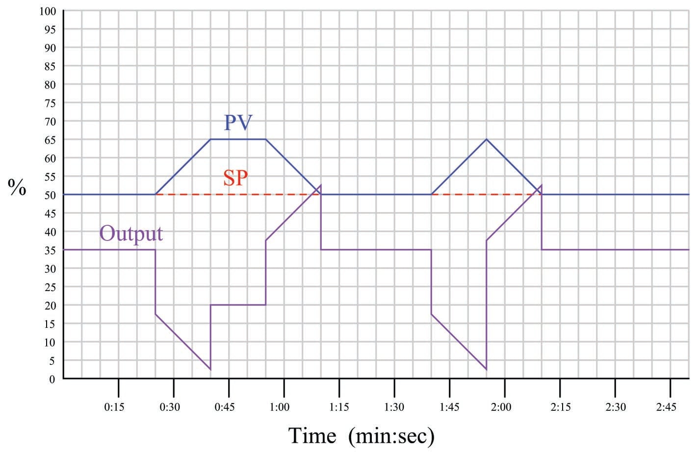
Suppose for example you were tasked with graphing the response of a PD (proportional + derivative) controller to the following PV and SP inputs over time. You are told the controller has a gain of 1, a derivative time constant of 0.3 minutes, and is reverse-acting:
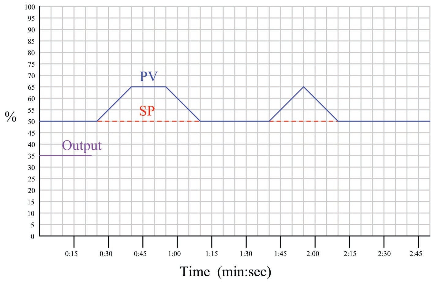
My first recommendation is to qualitatively sketch the individual P and D responses. Simply draw two different trends, each one right above or below the given PV/SP trends, showing the shapes of each response over time. You might even find it easier to do if you re-draw the original PV and SP trends on a piece of non-graph paper with the qualitative P and D trends also sketched on the same piece of non-graph paper. The purpose of the qualitative sketches is to separate the task of determining shapes from the task of determining numerical values, in order to simplify the process.
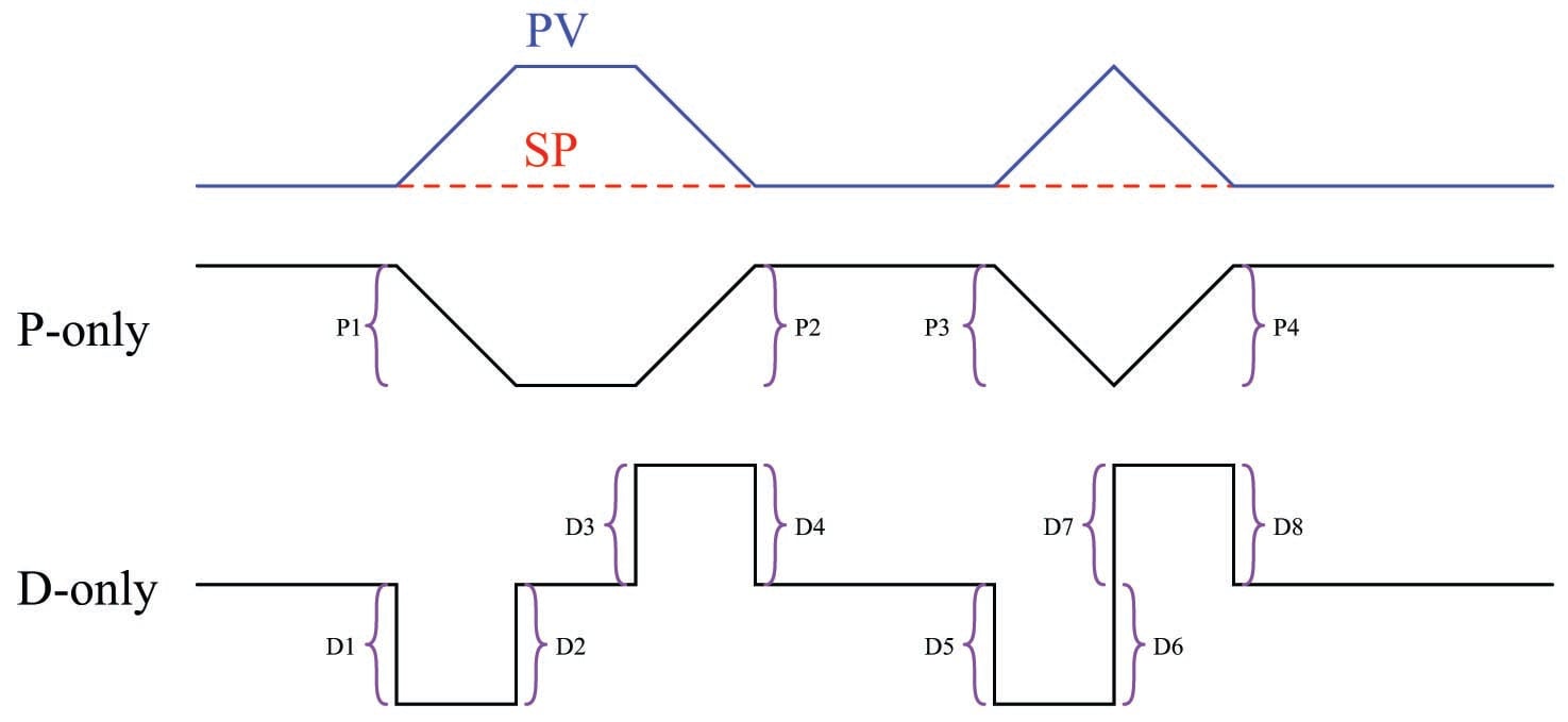
After sketching the separate P and D trends, label each one of the “features” (changes either up or down) in these qualitative trends. This will allow you to more easily combine the effects into one output trend later:
Now, you may qualitatively sketch an output trend combining each of these “features” into one graph. Be sure to label each ramp or step originating with the separate P or D trends, so you know where each “feature” of the combined output graph originates from:
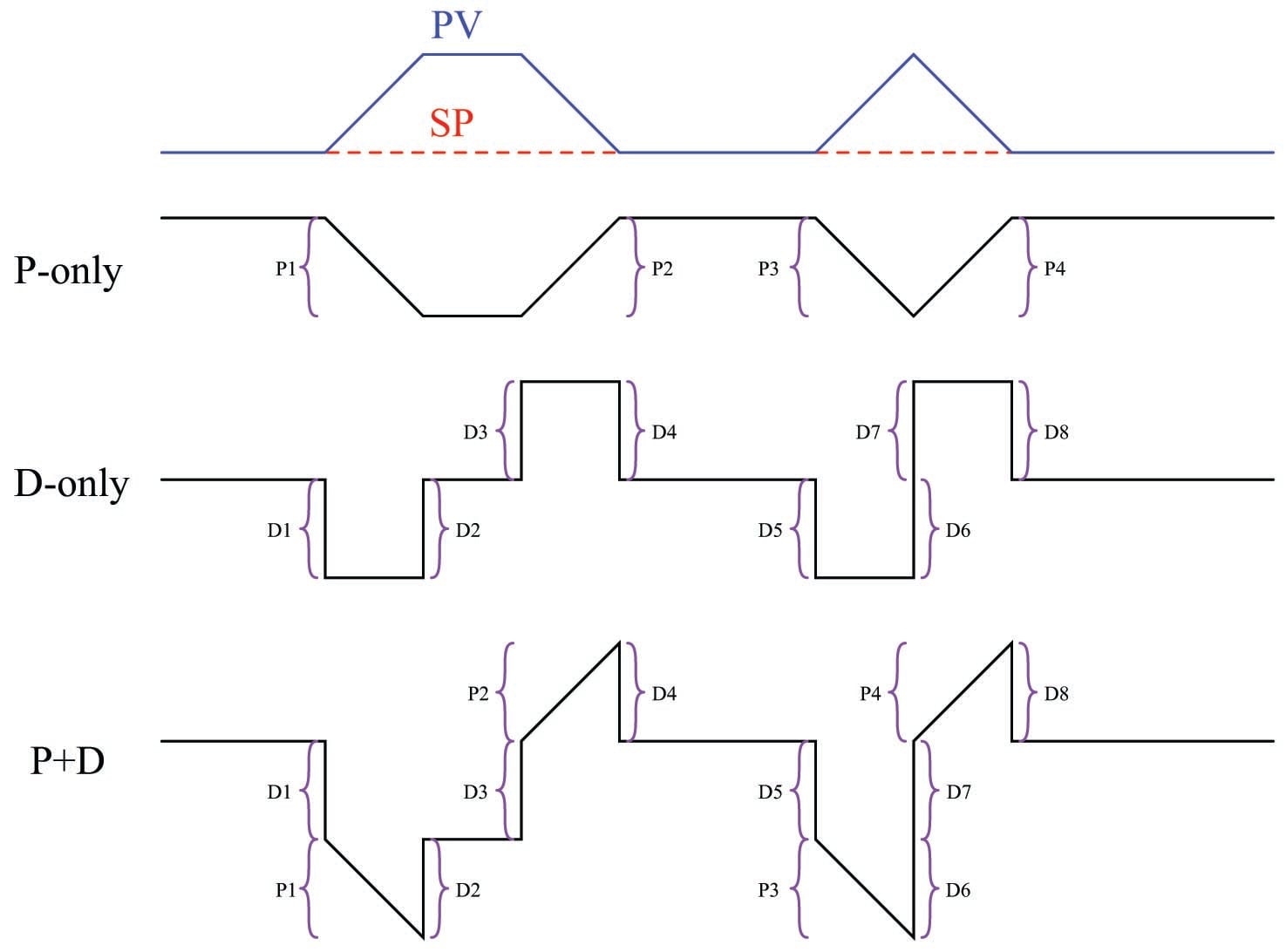
Once the general shape of the output has been qualitatively determined, you may go back to the separate P and D trends to calculate numerical values for each of the labeled “features.”
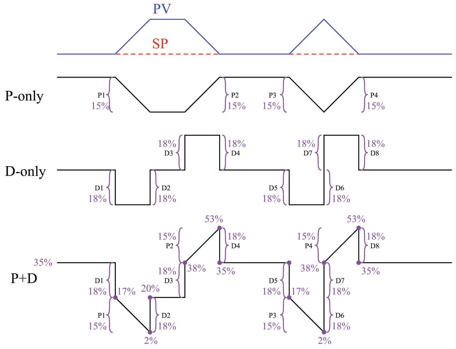
Note that each of the PV ramps is 15% in height, over a time of 15 seconds (one-quarter of a minute). With a controller gain of 1, the proportional response to each of these ramps will also be a ramp that is 15% in height.
Taking our given derivative time constant of 0.3 minutes and multiplying that by the PV’s rate-of-change (\(d\hbox{PV} \over dt\)) during each of its ramping periods (15% per one-quarter minute, or 60% per minute) yields a derivative response of 18% during each of the ramping periods. Thus, each derivative response “step” will be 18% in height.
Going back to the qualitative sketches of P and D actions, and to the combined (qualitative) output sketch, we may apply the calculated values of 15% for each proportional ramp and 18% for each derivative step to the labeled “features.” We may also label the starting value of the output trend as given in the original problem (35%), to calculate actual output values at different points in time. Calculating output values at specific points in the graph becomes as easy as cumulatively adding and subtracting the P and D “feature” values to the starting output value:
Now that we know the output values at all the critical points, we may quantitatively sketch the output trend on the original graph:
REVIEW:
-
System response is the combined reaction to any included P, I, and/or D tuning parameters.
-
Proportional response graph is the same as the shape of the input SP. Sudden change in setpoint = sudden equal change in P response.
-
Integral response graph increases as long as the SP is above PV, decreases as the SP is below the PV.
-
Larger difference between SP and PV (in other words, large changes) lead to a greater increase in integral response.
-
Derivative response only appears if the SP or PV is changing.
-
Rapid changes, no matter how large they are, lead to a large derivative response.
Interested in more PID and control system topics?
Related Worksheets:
- PID loop tuning
- Troubleshooting problems in control systems
- RTD and thermocouple circuits with millivolt calculations
Related Textbook Pages:
- Negative Consequences of Poor PID Controller Tuning
- Tuning PID Controllers
- Logic Programming in PLCs
Related Technical Articles:
- Using PID and Feedback Loops for Precise Motion Systems
- Proportional Gain and Proportional Band Explained
- Integral Windup Method in PID Control
