 Facebook
 Google
 GitHub
 Linkedin
PID Control Terminology
PID controllers are the complete physical or software objects that allow systems to respond to control inputs with just the right rate and accuracy to produce optimized operation.
PID control can be a confusing concept to understand. Here, a brief summary of each term within PID (P. I, and D) is presented for your learning benefit.
Proportional Control Mode (P)
Proportional – sometimes called gain or sensitivity – is a control action reproducing changes in input as changes in output. Proportional controller action responds to present changes in input by generating immediate and commensurate changes in output. When you think of “proportional action” (P), think prompt: this control action works immediately (never too soon or too late) to match changes in the input signal.
Mathematically defined, proportional action is the ratio of output change to input change. This may be expressed as a quotient of differences, or as a derivative (a rate of change, using calculus notation):
\[\hbox{Gain value} = {\Delta \hbox{Output} \over \Delta \hbox{Input}}\]
\[\hbox{Gain value} = {d\hbox{Output} \over d\hbox{Input}} = {dm \over de}\]
For example, if the PV input of a proportional-only process controller with a gain of 2 suddenly changes (“steps”) by 5 percent, and the output will immediately jump by 10 percent (\(\Delta\)Output = Gain \(\times\) \(\Delta\)Input). The direction of this output jump in relation to the direction of the input jump depends on whether the controller is configured for direct or reverse action.
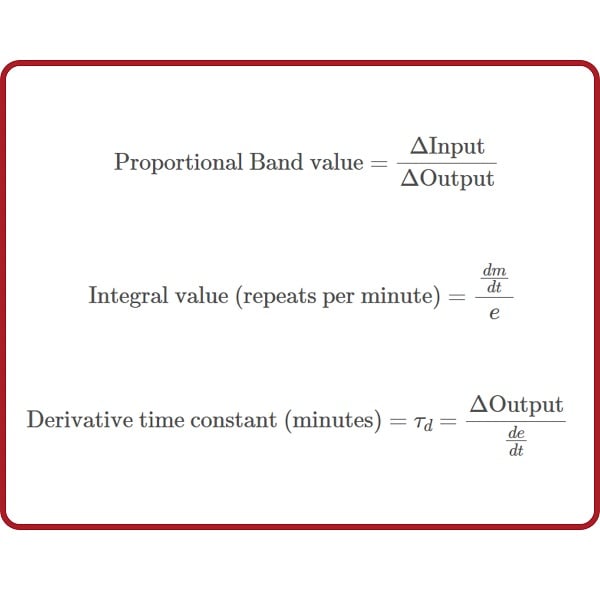
A legacy term used to express this same concept is proportional band: the mathematical reciprocal of gain. “Proportional band” is defined as the amount of input change necessary to evoke full-scale (100%) output change in a proportional controller. Incidentally, it is always expressed as a percentage, never as fraction or as a per unit value:
\[\hbox{Proportional Band value} = {\Delta \hbox{Input} \over \Delta \hbox{Output}}\]
\[\hbox{Proportional Band value} = {d\hbox{Input} \over d\hbox{Output}} = {de \over dm}\]
Using the same example of a proportional controller exhibiting an output “step” of 10% in response to a PV “step” of 5%, the proportional band would be 50%: the reciprocal of its gain (\({1 \over 2} = 50\%\)). Another way of saying this is that a 50% input “step” would be required to change the output of this controller by a full 100%, since its gain is set to a value of 2.
Integral Control Mode (I)
Integral – sometimes called reset or floating control – is a control action causing the output signal to change over time at a rate proportional to the amount of error (the difference between PV and SP values). Integral controller action responds to error accumulated over time, ramping the output signal are far as it needs to go to completely eliminate error. If proportional (P) action tells the output how far to move when an error appears, integral (I) action tells the output how fast to move when an error appears. If proportional (P) action acts on the present, integral (I) action acts on the past. Thus, how far the output signal gets driven by integral action depends on the history of the error over time: how much error existed, and for how long. When you think of “integral action” (I), think impatience: this control action drives the output further and further the longer PV fails to match SP.
Mathematically defined, integral action is the ratio of output velocity to input error:
\[\hbox{Integral value (repeats per minute)} = {\hbox{Output velocity} \over \hbox{Input error}}\]
\[\hbox{Integral value (repeats per minute)} = {{dm \over dt} \over e}\]
An alternate way to express integral action is to use the reciprocal unit of “minutes per repeat.” If we define integral action in these terms, the defining equations must be reciprocated:
\[\hbox{Integral time constant (minutes per repeat)} = \tau_i = {\hbox{Input error} \over \hbox{Output velocity}}\]
\[\hbox{Integral time constant (minutes per repeat)} = \tau_i = {e \over {dm \over dt}}\]
For example, if an error of 5% appears between PV and SP on an integral-only process controller with an integral value of 3 repeats per minute (i.e. an integral time constant of 0.333 minutes per repeat), the output will begin ramping at a rate of 15% per minute (\(dm \over dt\) = Integral_value \(\times\) \(e\), or \(dm \over dt\) = \(e \over \tau_i\)). In most PI and PID controllers, integral response is also multiplied by proportional gain, so the same conditions applied to a PI controller that happened to also have a gain of 2 would result in an output ramping rate of 30% per minute (\(dm \over dt\) = Gain_value \(\times\) Integral_value \(\times\) \(e\), or \(dm \over dt\) = Gain_value \(\times\) \(e \over \tau_i\)). The direction of this ramping in relation to the direction (sign) of the error depends on whether the controller is configured for direct or reverse action.
Derivative Control Mode (D)
Derivative – sometimes called rate or pre-act – is a control action causing the output signal to be offset by an amount proportional to the rate at which the input is changing. Derivative controller action responds to how quickly the input changes over time, biasing the output signal commensurate with that rate of input change. If proportional (P) action tells the output how far to move when an error appears, derivative (D) action tells the output how far to move when the input ramps. If proportional (P) action acts on the present and integral (I) action acts on the past, derivative (D) action acts on the future: it effectively “anticipates” overshoot by tempering the output response according to how fast the process variable is rising or falling. When you think of “derivative action” (D), think discretion: this control action is cautious and prudent, working against change.
Mathematically defined, derivative action is the ratio of output offset to input velocity:
\[\hbox{Derivative time constant (minutes)} = \tau_d = {\hbox{Output offset} \over \hbox{Input velocity}}\]
\[\hbox{Derivative time constant (minutes)} = \tau_d = {\Delta \hbox{Output} \over {de \over dt}}\]
For example, if the PV signal begins to ramp at a rate of 5% per minute on a process controller with a derivative time constant of 4 minutes, the output will immediately become offset by 20% (\(\Delta\)Output = Derivative_value \(\times\) \(de \over dt\)). In most PD and PID controllers, derivative response is also multiplied by proportional gain, so the same conditions applied to a PD controller that happened to also have a gain of 2 would result in an immediate offset of 40% (\(\Delta\)Output = Gain_value \(\times\) Derivative_value \(\times\) \(de \over dt\)). The direction (sign) of this offset in relation to the direction of the input ramping depends on whether the controller is configured for direct or reverse action.
REVIEW:
-
Error is defined as ‘the difference between the setpoint and the current actual process value.’
-
Proportional control acts on the current error value alone.
-
Integral control acts on the accumulated error over a period of time.
-
Derivative control acts on the rate of change (speed) of the error, or of the process variable itself.
Interested in more PID and control system topics?
Related Worksheets:
- PID loop tuning
- Troubleshooting problems in control systems
- RTD and thermocouple circuits with millivolt calculations
Related Textbook Pages:
- Negative Consequences of Poor PID Controller Tuning
- Tuning PID Controllers
- Logic Programming in PLCs
Related Technical Articles:
- Using PID and Feedback Loops for Precise Motion Systems
- Proportional Gain and Proportional Band Explained
- Integral Windup Method in PID Control
