 Facebook
 Google
 GitHub
 Linkedin
Analog Electronic PID Controllers

Can you build a PID controller using only analog components?
Constructing PID control systems using discrete components is a fairly simple method involving operational amplifiers (op amps), resistors, and capacitors. This strategy, however, is becoming less common due to the ever-lowering costs of digital controllers.
Although analog electronic process controllers are considered a newer technology than pneumatic process controllers, they are actually “more obsolete” than pneumatic controllers. Panel-mounted (inside a control room environment) analog electronic controllers were a great improvement over panel-mounted pneumatic controllers when they were first introduced to industry, but they were superseded by digital controller technology later on. Field-mounted pneumatic controllers were either replaced by panel-mounted electronic controllers (either analog or digital) or left alone. Applications still exist for field-mounted pneumatic controllers, even now at the beginning of the 21\(^{st}\) century, but very few applications exist for analog electronic controllers in any location.
Analog electronic controllers enjoy two inherent advantages over digital electronic controllers: greater reliability and faster response. However, these advantages have been diminishing as digital control technology has advanced. Today’s digital electronic technology is far more reliable than the digital technology available during the heyday of analog electronic controllers. Now that digital controls have achieved very high levels of reliability, the first advantage of analog control is largely academic, leaving only the second advantage for practical consideration. The advantage of faster speed may be fruitful in applications such as motion control, but for most industrial processes even the slowest digital controller is fast enough. Furthermore, the numerous advantages offered by digital technology (data recording, networking capability, self-diagnostics, flexible configuration, function blocks for implementing different control strategies) severely weaken the relative importance of reliability and speed.
Operational Amplifier (Op Amp) PID Controllers
Most analog electronic PID controllers utilize operational amplifiers in their designs. It is relatively easy to construct circuits performing amplification (gain), integration, differentiation, summation, and other useful control functions with just a few opamps, resistors, and capacitors.
Proportional Controller Circuit
The basic proportional-only control algorithm follows this formula:
\[m = K_p e + b\]
Where,
\(m\) = Controller output
\(e\) = Error (difference between PV and SP)
\(K_p\) = Proportional gain
\(b\) = Bias
The “error” variable (\(e\)) is the mathematical difference between process variable and setpoint. If the controller is direct-acting, \(e\) = PV \(-\) SP. If the controller is reverse-acting, \(e\) = SP \(-\) PV. Thus,
\[m = K_p (\hbox{PV} - \hbox{SP}) + b \hskip 30pt \hbox{Direct-acting}\]
\[m = K_p (\hbox{SP} - \hbox{PV}) + b \hskip 30pt \hbox{Reverse-acting}\]
Mathematical operations such as subtraction, multiplication by a constant, and addition are quite easy to perform using analog electronic (operational amplifier) circuitry. Prior to the advent of reliable digital electronics for industrial applications, it was natural to use analog electronic circuitry to perform proportional control for process control loops.
For example, the subtraction function necessary to calculate error (\(e\)) from process variable and setpoint signals may be performed with a three-amplifier “subtractor” circuit:
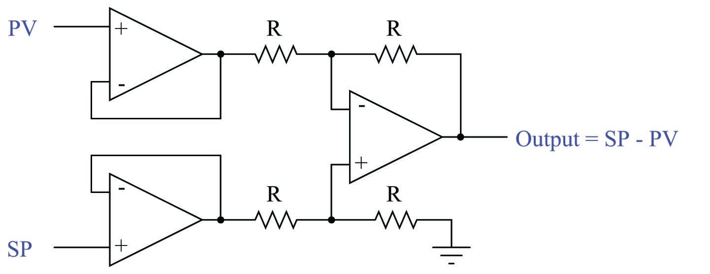
This particular subtractor circuit calculates error for a reverse-acting controller. As the PV signal increases, the error signal decreases (becomes more negative). It could be modified for direct action simply by swapping the two inputs: SP on top and PV on bottom such that the Output becomes PV \(-\) SP.
Op Amp Proportional Controller Gain
Gain is really nothing more than multiplication by a constant, in this case the constant being \(K_p\). A very simple one-amplifier analog circuit for performing this multiplication is the inverting amplifier circuit:
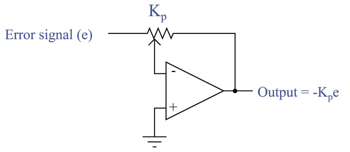
With the potentiometer’s wiper in mid-position, the voltage gain of this circuit will be 1 (with an inverted polarity which we shall ignore for now). Moving the wiper toward the left-hand side of the potentiometer increases the circuit’s gain past unity, while moving the wiper toward the right-hand side of the potentiometer decreases the gain toward zero.
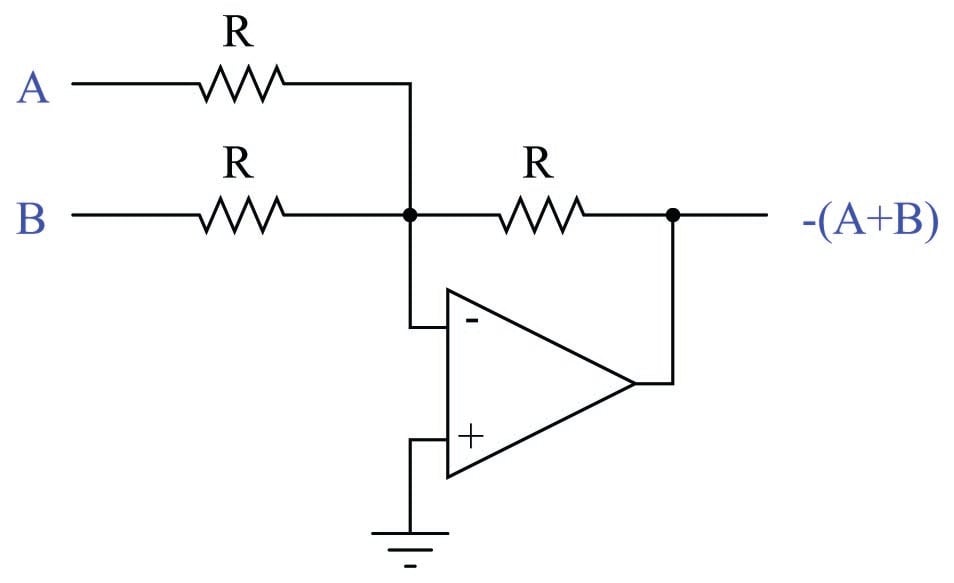
In order to add the bias (\(b\)) term in the proportional control equation, we need an analog circuit capable of summing two voltage signals. This need is nicely met in the inverting summing circuit, shown here:
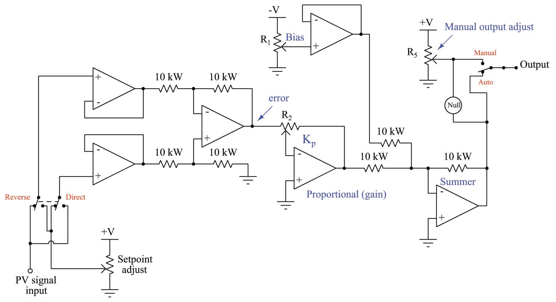
Combining all these analog functions together into one circuit, and adding a few extra features such as direct/reverse action selection, bias adjustment, and manual control with a null voltmeter to facilitate bumpless mode transfer, gives us this complete analog electronic proportional controller:
Derivative Controller Circuit
Differentiating and integrating live voltage signals with respect to time is quite simple using operational amplifier circuits. Instead of using all resistors in the negative feedback network, we may implement these calculus functions by using a combination of capacitors and resistors, exploiting the capacitor’s natural derivative relationship between voltage and current:
\[I = C {dV \over dt}\]
Where,
\(I\) = Current through the capacitor (amperes)
\(C\) = Capacitance of capacitor (farads)
\(V\) = Voltage across the capacitor (volts)
\(dV \over dt\) = Rate-of-change of voltage across the capacitor (volts per second)
If we build an operational amplifier with a resistor providing negative feedback current through a capacitor, we create a differentiator circuit where the output voltage is proportional to the rate-of-change of the input voltage:
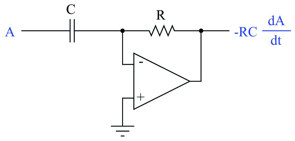
Since the inverting input of the operational amplifier is held to ground potential by feedback (a “virtual ground”), the capacitor experiences the full input voltage of signal \(A\). So, as \(A\) varies over time, the current through that capacitor will directly represent the signal \(A\)’s rate of change over time (\(I = C{dA \over dt}\)). This current passes through the feedback resistor, creating a voltage drop at the output of the amplifier directly proportional to signal \(A\)’s rate of change over time. Thus, the output voltage of this circuit reflects the input voltage’s instantaneous rate of change, albeit with an inverted polarity. The mathematical term \(RC\) is the time constant of this circuit. For a differentiator circuit such as this, we typically symbolize its time constant as \(\tau_d\) (the “derivative” time constant).
For example, if the input voltage to this differentiator circuit were to ramp at a constant rate of +4.3 volts per second (rising) with a resistor value of 10 k\(\Omega\) and a capacitor value of 33 \(\mu\)F (i.e. \(\tau_d\) = 0.33 seconds), the output voltage would be a constant \(-1.419\) volts:
\[V_{out} = -RC {dV_{in} \over dt}\]
\[V_{out} = -(10000 \> \Omega)(33 \times 10^{-6} \hbox{ F}) \left({4.3 \hbox{ V} \over \hbox{s}}\right)\]
\[V_{out} = -(0.33 \hbox{ s}) \left({4.3 \hbox{ V} \over \hbox{s}}\right)\]
\[V_{out} = -1.419 \hbox{ V}\]
Recall that the purpose of derivative action in a PID controller is to react to sudden changes in either the error (\(e\)) or the process variable (PV). This circuit fulfills that function, by generating an output proportional to the input voltage’s rate of change.
Integral Controller Circuit
If we simply swap the locations of the resistor and capacitor in the feedback network of this operational amplifier circuit, we create an integrator circuit where the output voltage rate-of-change is proportional to the input voltage:
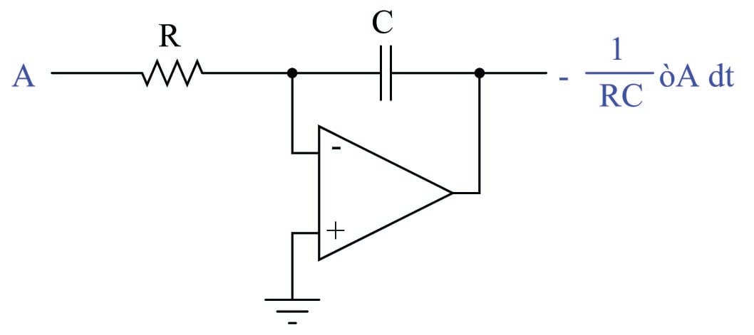
This integrator circuit provides the exact inverse function of the differentiator. Rather than a changing input signal generating an output signal proportional to the input’s rate of change, an input signal in this circuit controls the rate at which the output signal changes.
The way it works is by acting as a current source, pumping current into the capacitor at a value determined by the input voltage and the resistor value. Just as in the previous (differentiator) circuit where the inverting terminal of the amplifier was a “virtual ground” point, the input voltage in this circuit is impressed across the resistor \(R\). This creates a current which must go through capacitor \(C\) on its way either to or from the amplifier’s output terminal. As we have seen in the capacitor’s equation (\(I = C {dV \over dt}\)), a current forced through a capacitor causes the capacitor’s voltage to change over time. This changing voltage becomes the output signal of the integrator circuit. As in the case of the differentiator circuit, the mathematical term \(RC\) is the time constant of this circuit as well. Being an integrator, we customarily represent this “integral” time constant as \(\tau_i\).
Any amount of change in output voltage (\(\Delta V_{out}\)) occurring between some initial time (\(t_0\)) and a finishing time (\(t_f\)) may be calculated by the following integral:
\[\Delta V_{out} = -{1 \over RC} \int_{t_0}^{t_f} V_{in} \> dt\]
If we wish to know the absolute output voltage at the end of that time interval, all we need to do is add the circuit’s initial output voltage (\(V_0\), i.e. the voltage stored in the capacitor at the initial time \(t_0\)) to the calculated change:
\[V_{out} = -{1 \over RC} \int_{t_0}^{t_f} V_{in} \> dt + V_0\]
For example, if we were to input a constant DC voltage of +1.7 volts to this circuit with a resistor value of 81 k\(\Omega\) and a capacitor value of 47 \(\mu\)F (i.e. \(\tau_i\) = 3.807 seconds), the output voltage would ramp at a constant rate of \(-0.447\) volts per second. If the output voltage were to begin at \(-3.0\) volts and be allowed to ramp for exactly 12 seconds at this rate, it would reach a value of \(-8.359\) volts at the conclusion of that time interval:
\[V_{out} = -{1 \over RC} \int_{t_{0}}^{t_{f}} V_{in} \> dt + V_0\]
\[V_{out} = -\left({1 \over (81000 \> \Omega)(47 \times 10^{-6} \hbox{ F})}\right) \left(\int_0^{12} 1.7 \hbox{ V} \> dt \right) - 3 \hbox{ V}\]
\[V_{out} = -\left({1 \over 3.807 \hbox{ s}}\right) (20.4 \hbox{ V} \cdot \hbox{s}) - 3 \hbox{ V}\]
\[V_{out} = - 5.359 \hbox{ V} - 3 \hbox{ V}\]
\[V_{out} = - 8.359 \hbox{ V}\]
If, after ramping for some amount of time, the input voltage of this integrator circuit is brought to zero, the integrating action will cease. The circuit’s output will simply hold at its last value until another non-zero input signal voltage appears.
Recall that the purpose of integral action in a PID controller is to eliminate offset between process variable and setpoint by calculating the error-time product (how far PV deviates from SP, and for how long). This circuit will fulfills that function if the input voltage is the error signal, and the output voltage contributes to the output signal of the controller.
Complete PID Controller Circuit Design
The following schematic diagram shows a full PID controller implemented using eight operational amplifiers, designed to input and output voltage signals representing PV, SP, and Output:
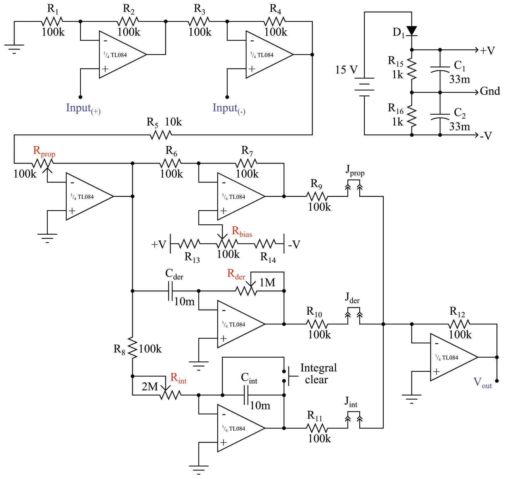
It is somewhat stunning to realize that such a controller, fully capable of controlling many industrial process types, may be constructed using only two integrated circuit “chips” (two “quad” operational amplifiers) and a handful of passive electronic components. The only significant engineering challenge in this simple circuit design is achieving slow enough time constants (in the range of minutes rather than seconds) in the integrator and differentiator functions using non-polarized capacitors.
Ideal PID Equation
This controller implements the so-called ideal PID algorithm, with the proportional (gain) value distributing to the integral and derivative terms:
\[m = K_p \left(e + {1 \over \tau_i} \int e \> dt + \tau_d {de \over dt} \right) \hbox{\hskip 50pt Ideal PID equation}\]
We may determine this from the schematic diagram by noting that the I and D functions each receive their input signals from the output of the proportional amplifier (the one with the \(R_{prop}\) potentiometer). Adjusting \(R_{prop}\) affects not only the controller’s proportional gain, but also the sensitivity of \(\tau_i\) and \(\tau_d\).
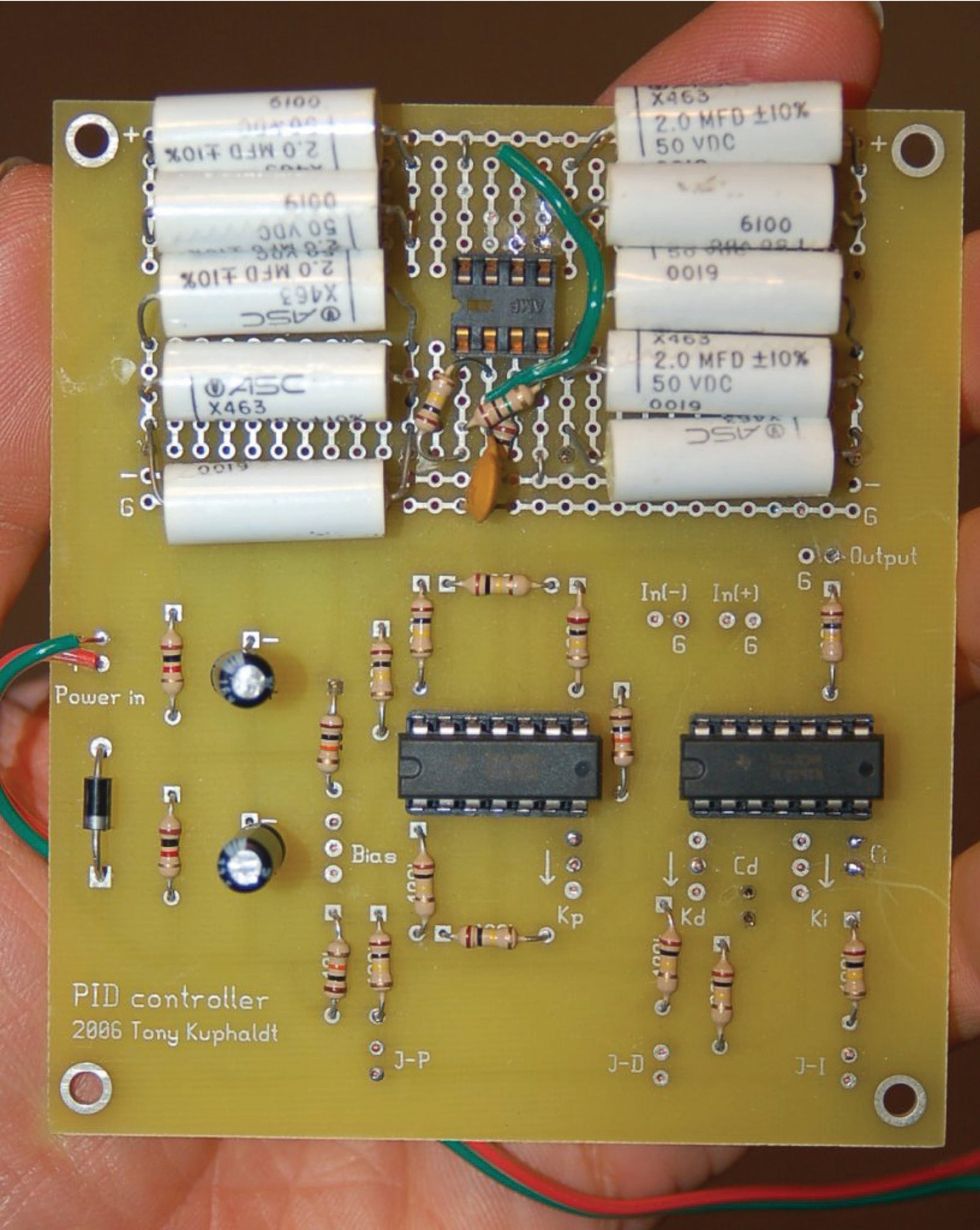
An actual implementation of this PID controller in printed circuit board form appears here:
It is possible to construct an analog PID controller with fewer components. An example is shown here:
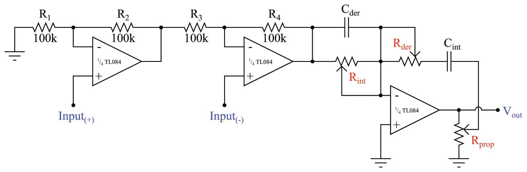
As you can see, a single operational amplifier does all the work of calculating proportional, integral, and derivative responses. The first two amplifiers do nothing but buffer the input signals and calculate error (PV \(-\) SP, or SP \(-\) PV, depending on the direction of action).
One of the consequences of consolidating all three control terms in a single amplifier is that those control terms interact with each other. The mathematical expression of this control action is shown here, called the series or interacting PID equation:
\[m = K_p \left[ \left({\tau_d \over \tau_i} + 1 \right) e + {1 \over \tau_i} \int e \> dt + \tau_d {de \over dt} \right] \hbox{\hskip 25pt Series or Interacting PID equation}\]
Not only does a change in gain (\(K_p\)) alter the relative responses of integral and derivative in the series equation (as it also does in the ideal equation), but changes in either integral or derivative time constants also have an effect on proportional response! This is especially noticeable when the integral time constant is set to some very small value, which is typically the case on fast-responding, self-regulating processes such as liquid flow or liquid pressure control.
It should be apparent that an analog controller implementing the series equation is simpler in construction than one implementing either the parallel or ideal PID equation. This also happens to be true for pneumatic PID controller mechanisms: the simplest analog controller designs all implement the series PID equation.
Examples of a Single-loop Analog PID Controller
Foxboro
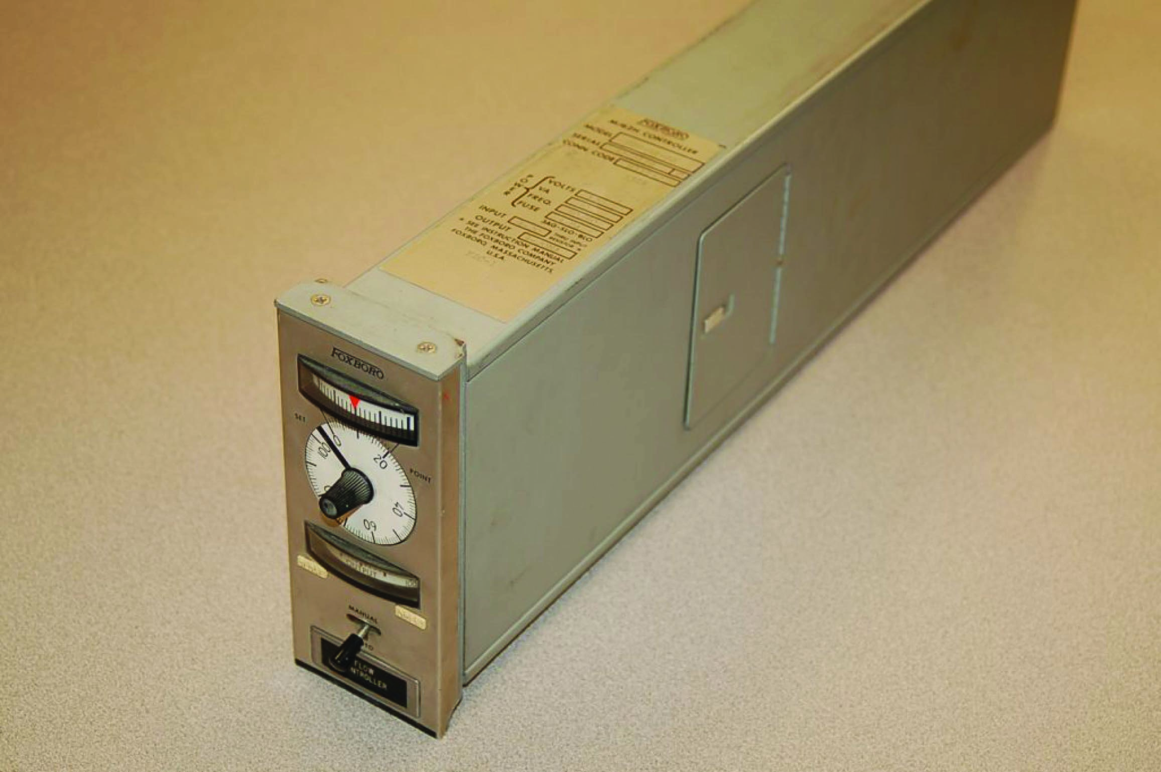
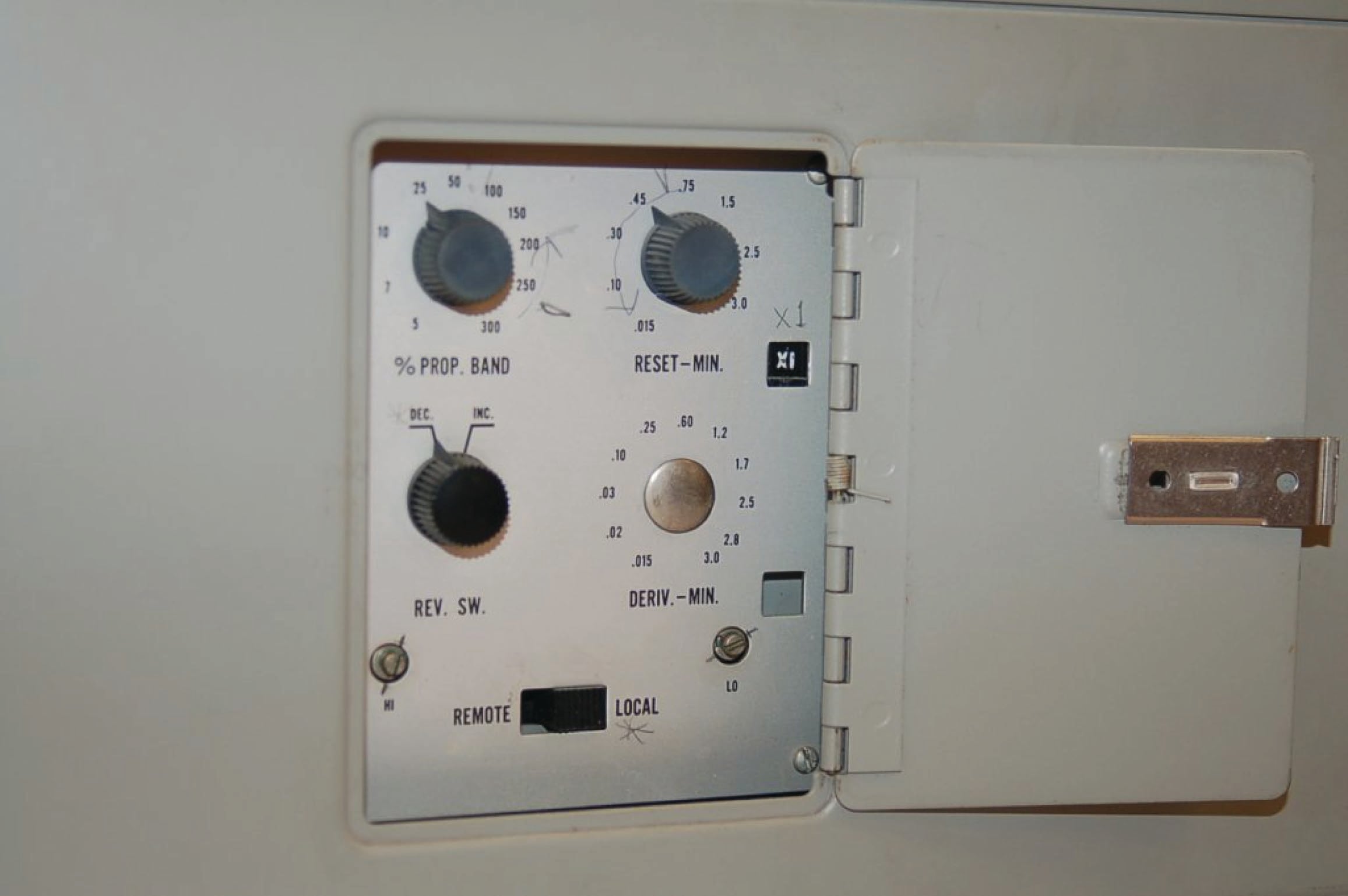
One popular analog electronic controller was the Foxboro model 62H, shown in the following photographs. Like the model 130 pneumatic controller, this electronic controller was designed to fit into a rack next to several other controllers. Tuning parameters were adjustable by moving potentiometer knobs under a side-panel accessible by partially removing the controller from its rack:
Fisher
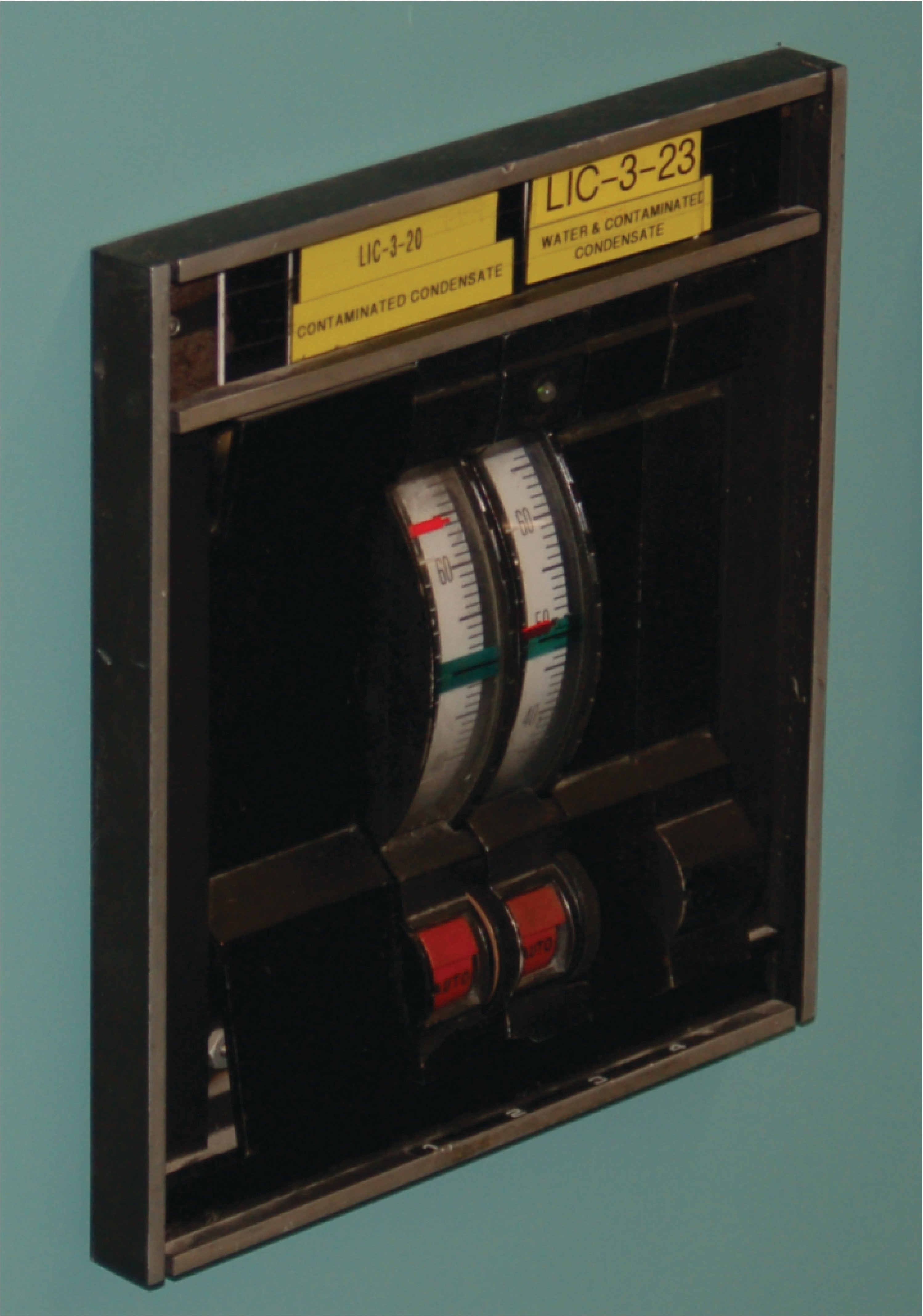
The Fisher corporation manufactured a series of analog electronic controllers called the AC\(^{2}\), which were similar in construction to the Foxboro model 62H, but very narrow in width so that many could be fit into a compact panel space. Here we see a pair of Fisher AC\(^{2}\) controllers mounted side-by-side in the same rack, used to control liquid level in a pulping process:
Like the pneumatic panel-mounted controllers preceding, and digital panel-mount controllers to follow, the tuning parameters for a panel-mounted analog electronic controller were typically accessed on the controller’s side. The controller could be slid partially out of the panel to reveal the P, I, and D adjustment knobs (as well as direct/reverse action switches and other configuration controls).
Indicators on the front of an analog electronic controller served to display the process variable (PV), setpoint (SP), and manipulated variable (MV, or output) for operator information. Many analog electronic controllers did not have separate meter indications for PV and SP, but rather used a single meter movement to display the error signal, or difference between PV and SP. On the Foxboro model 62H, a hand-adjustable knob provided both indication and control over SP, while a small edge-reading meter movement displayed the error. A negative meter indication showed that the PV was below setpoint, and a positive meter indication showed that the PV was above setpoint.
The Fisher AC\(^{2}\) analog electronic controller used the same basic technique, cleverly applied in such a way that the PV was displayed in real engineering units. The setpoint adjustment was a large wheel, mounted so the edge faced the operator. Along the circumference of this wheel was a scale showing the process variable range, from the LRV at one extreme of the wheel’s travel to the URV at the other extreme of the wheel’s travel. The actual setpoint value was the middle of the wheel from the operator’s view of the wheel edge. A single meter movement needle traced an arc along the circumference of the wheel along this same viewable range. If the error was zero (PV = SP), the needle would be positioned in the middle of this viewing range, pointed at the same value along the scale as the setpoint. If the error was positive, the needle would rise up to point to a larger (higher) value on the scale, and if the error was negative the needle would point to a smaller (lower) value on the scale. For any fixed value of PV, this error needle would therefore move in exact step with the wheel as it was rotated by the operator’s hand. Thus, a single adjustment and a single meter movement displayed both SP and PV in very clear and unambiguous form.
Taylor
Taylor manufactured a line of analog panel-mounted controllers that worked much the same way, with the SP adjustment being a graduated tape reeled to and fro by the SP adjustment knob. The middle of the viewable section of tape (as seen through a plastic window) was the setpoint value, and a single meter movement needle pointed to the PV value as a function of error. If the error happened to be zero (PV = SP), the needle would point to the middle of this viewable section of tape, which was the SP value.
Moore Syncro
Another popular panel-mounted analog electronic controller was the Moore Syncro, which featured plug-in modules for implementing different control algorithms (different PID equations, nonlinear signal conditioning, etc.). These plug-in function modules were a hardware precursor to the software “function blocks” appearing in later generations of digital controllers: a simple way of organizing controller functionality so that technicians unfamiliar with computer programming could easily configure a controller to do different types of control functions. Later models of the Syncro featured fluorescent bargraph displays of PV and SP for easy viewing in low-light conditions.
Analog single-loop controllers are largely a thing of the past, with the exception of some low-cost or specialty applications. An example of the former is shown here, a simple analog temperature controller small enough to fit in the palm of my hand:
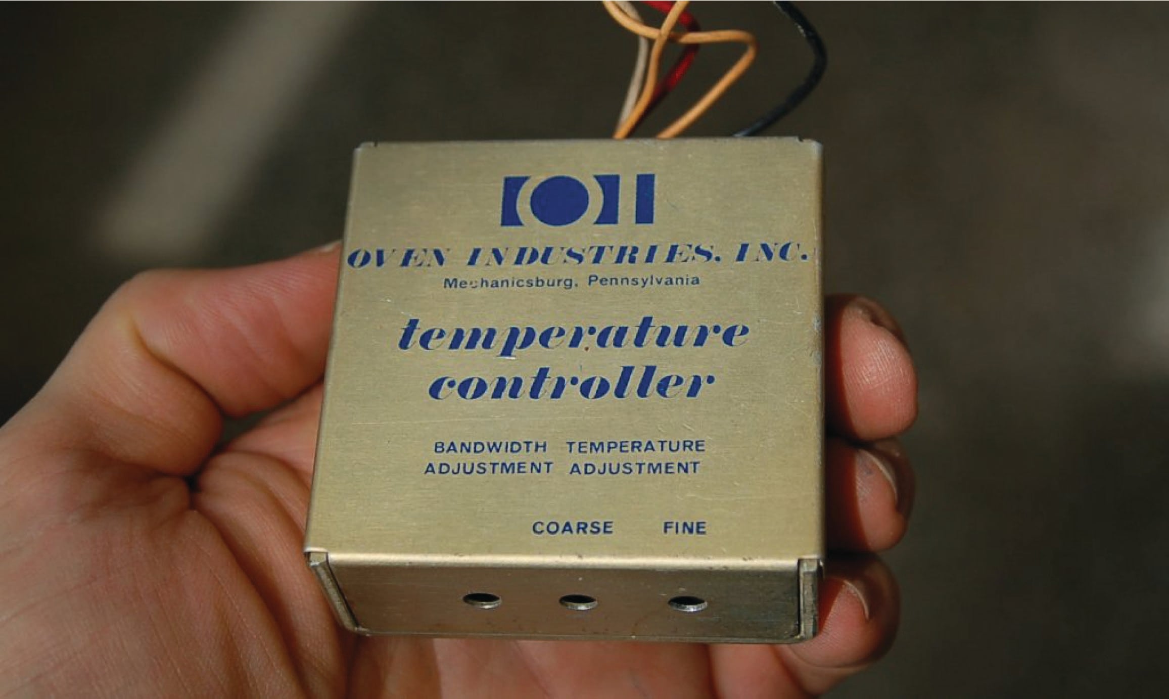
This particular controller happened to be part of a sulfur dioxide analyzer system, controlling the internal temperature of a gas regulator panel to prevent vapors in the sample stream from condensing in low spots of the tubing and regulator system. The accuracy of such a temperature control application was not critical – if temperature was regulated to \(\pm\) 5 degrees Fahrenheit it would be more than adequate. This is an application where an analog controller makes perfect sense: it is very compact, simple, extremely reliable, and inexpensive. None of the features associated with digital PID controllers (programmability, networking, precision) would have any merit in this application.
Examples of a Multi-loop Analog Control System
In contrast to single-loop analog controllers, multi-loop systems control dozens or even hundreds of process loops at a time. Prior to the advent of reliable digital technology, the only electronic process control systems capable of handling the numerous loops within large industrial installations such as power generating plants, oil refineries, and chemical processing facilities were analog systems, and several manufacturers produced multi-loop analog systems just for these large-scale control applications.
Foxboro
One of the most technologically advanced analog electronic products manufactured for industrial control applications was the Foxboro SPEC 200 system. Although the SPEC 200 system used panel-mounted indicators, recorders, and other interface components resembling panel-mounted control systems, the actual control functions were implemented in a separate equipment rack which Foxboro called a nest. Printed circuit boards plugged into each “nest” provided all the control functions (PID controllers, alarm units, integrators, signal selectors, etc.) necessary, with analog signal wires connecting the various functions together with panel-mounted displays and with field instruments to form a working system.
Analog field instrument signals (4-20 mA, or in some cases 10-50 mA) were all converted to a 0-10 VDC range for signal processing within the SPEC 200 nest. Operational amplifiers (mostly the model LM301) formed the “building blocks” of the control functions, with a \(\pm\) 15 VDC power supply providing DC power for everything to operate.
The following photographs show a model 2AX+A4 proportional-integral (PI) controller card for a SPEC 200 system inserted into a metal frame (called a “module” by Foxboro). This module was designed to fit into a slot in a SPEC 200 “nest” where it would reside alongside many other similar cards, each card performing its own control function:
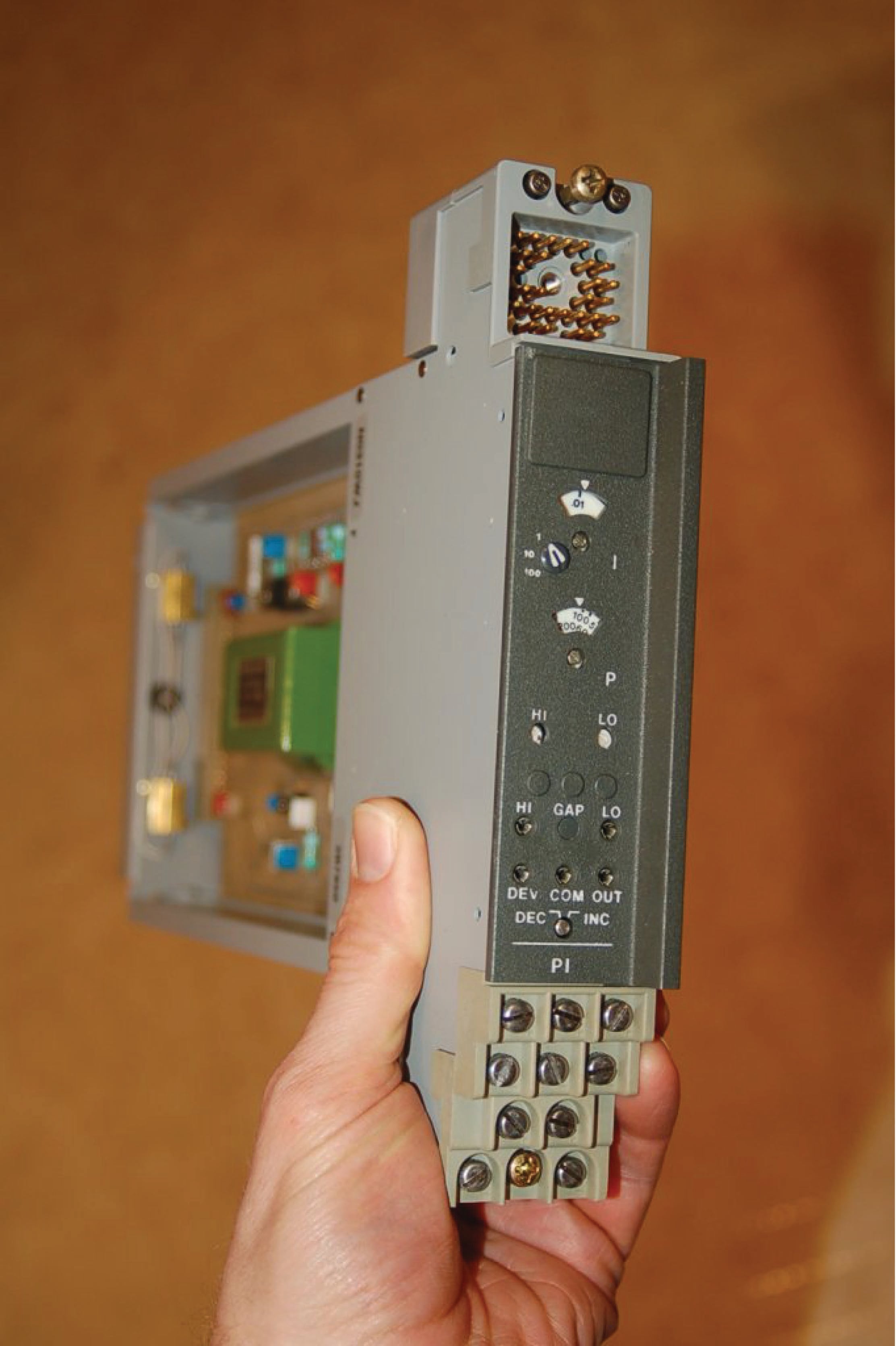
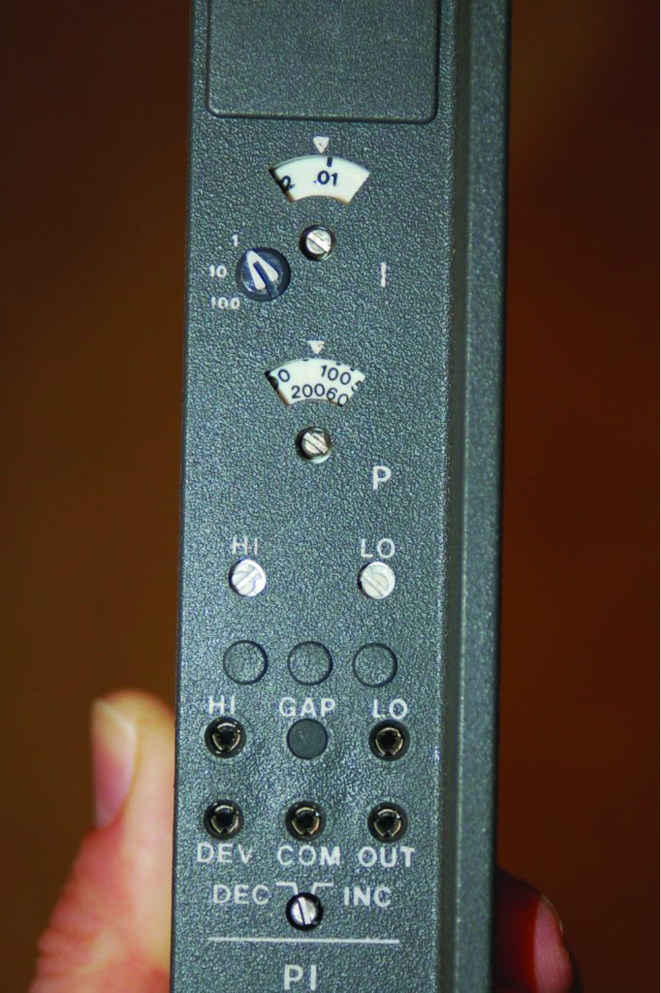
Tuning and alarm adjustments may be seen in the right-hand photograph. This particular controller is set to a proportional band value of approximately 170%, and an integral time constant of just over 0.01 minutes per repeat. A two-position rotary switch near the bottom of the card selected either reverse (“Dec”) or direct (“Inc”) control action.
The array of copper pins at the top of the module form the male half of a cable connector, providing connection between the control card and the front-panel instrument accessible to operations personnel. Since the tuning controls appear on the face of this controller card (making it a “card tuned” controller), they were not accessible to operators but rather only to the technical personnel with access to the nest area. Other versions of controller cards (“control station tuned”) had blank places where the P and I potentiometer adjustments appear on this model, with tuning adjustments provided on the panel-mounted instrument displays for easier access to operators.
The set of ten screw terminals at the bottom of the module provided connection points for the input and output voltage signals. The following list gives the general descriptions of each terminal pair, with the descriptions for this particular P + I controller written in italic type:
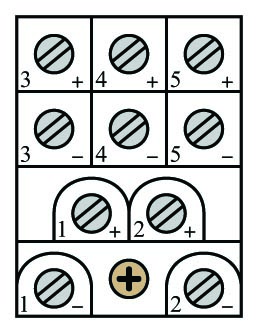
- Terminals (1+) and (1\(-\)): Input signal #1 (Process variable input)
- Terminals (2+) and (2\(-\)): Output signal #1 (Manipulated variable output)
- Terminals (3+) and (3\(-\)): Input #2, Output #4, or Option #1 (Remote setpoint)
- Terminals (4+) and (4\(-\)): Input #3, Output #3, or Option #2 (Optional alarm)
- Terminals (5+) and (5\(-\)): Input #4, Output #2, or Option #3 (Optional 24 VAC)
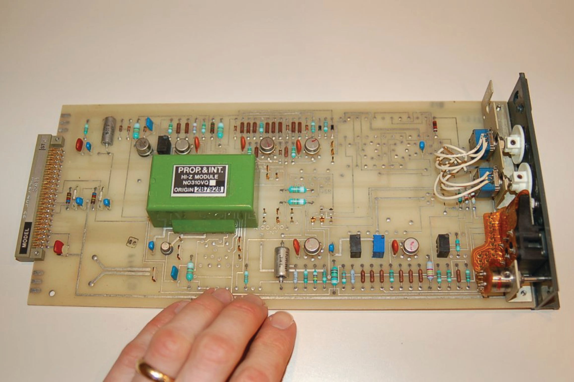
A photograph of the printed circuit board (card) removed from the metal module clearly shows the analog electronic components:
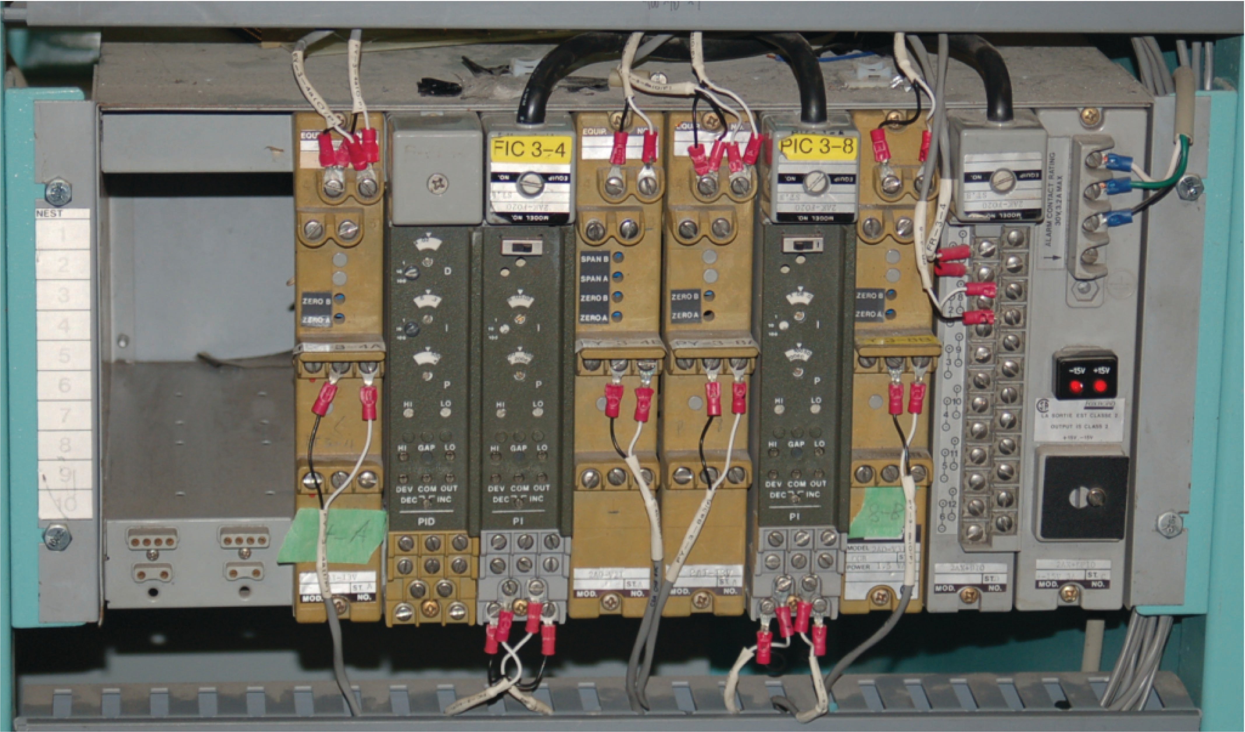
The following photograph shows a set of functioning Foxboro SPEC 200 controller modules residing in a “nest,” used to control a flow loop and a pressure loop in a wood pulping process. Both active controller modules are P + I units. An unused PID module resides just to the left of the flow controller module:
Foxboro engineers went to great lengths in their design process to maximize reliability of the SPEC 200 system, already an inherently reliable technology by virtue of its simple, analog nature. As a result, the reliability of SPEC 200 control systems is the stuff of legend.
REVIEW:
-
Analog PID control circuits begin with an op-amp ‘subtractor’ to calculate the error: setpoint signal (SP) - process variable (PV).
-
A single op-amp and potentiometer forms the proportional controller, or amplifier.
-
Offset bias can be added with a summing circuit.
-
Derivative (rate) control uses an RC time constant amplifier, as only a difference in potential will lead to a signal through a capacitor.
-
Integral (accumulated) control rearranges the RC circuit, so that only as the capacitor charges over time will the op-amp circuit respond.
Interested in more PID and control system topics?
Related Worksheets:
- PID loop tuning
- Troubleshooting problems in control systems
- RTD and thermocouple circuits with millivolt calculations
Related Textbook Pages:
- Negative Consequences of Poor PID Controller Tuning
- Tuning PID Controllers
- Logic Programming in PLCs
Related Technical Articles:
- Using PID and Feedback Loops for Precise Motion Systems
- Proportional Gain and Proportional Band Explained
- Integral Windup Method in PID Control
