 Facebook
 Google
 GitHub
 Linkedin
Control Valve Sizing
When control valves operate between fully open and fully shut, they serve much the same purpose in process systems as resistors do in electric circuits: to dissipate energy. Like resistors, the form that this dissipated energy takes is mostly heating, although some of the dissipated energy manifests in the form of vibration and noise.
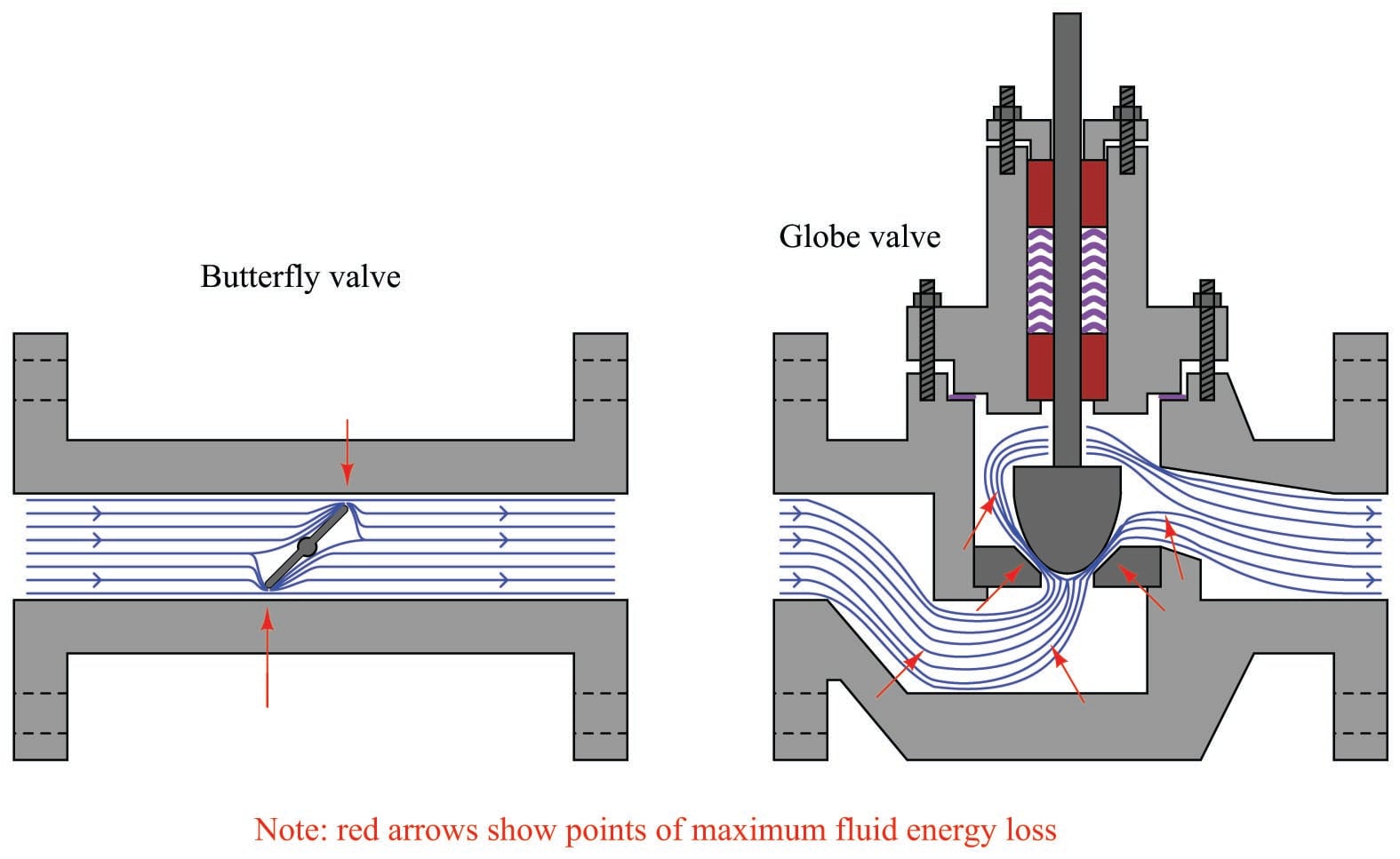
In most control valves, the dominant mechanism of energy dissipation comes as a result of turbulence introduced to the fluid as it travels through constrictive portions of the valve trim. The following illustration shows these constrictive points within two different control valve types (shown by arrows):
The act of choosing an appropriate control valve for the expected energy dissipation is called valve sizing.
Physics of Energy Dissipation in a Turbulent Fluid Stream
Control valves are rated in their ability to throttle fluid flow much in the same way resistors are rated in their ability to throttle the flow of electrons in a circuit. For resistors, the unit of measurement for electron flow restriction is the ohm: 1 ohm of resistance results in a voltage drop of 1 volt across that resistance given current through the resistance equal to 1 ampere:
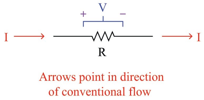
The mathematical relationship between current, voltage and resistance for any resistor is Ohm’s Law:
\[R = {V \over I}\]
Where,
\(R\) = Electrical resistance in ohms
\(V\) = Electrical voltage drop in volts
\(I\) = Electrical current in amperes
Ohm’s Law is a simple, linear relationship, expressing the “friction” encountered by electric charge carriers as they slowly drift through a solid object.
When a fluid moves turbulently through any restriction, energy is inevitably dissipated in that turbulence. The amount of energy dissipated is proportional to the kinetic energy of the turbulent motion, which is proportional to the square of velocity according to the classic kinetic energy equation for moving objects:
\[E_k = {1 \over 2} mv^2\]
If we were to re-write this equation to express the amount of kinetic energy represented by a volume of moving fluid with velocity \(v\), it would look like this:
\[\hbox{Kinetic energy per unit volume} = {1 \over 2} \rho v^2\]
We know that the amount of energy dissipated by turbulence in such a fluid stream will be some proportion (\(k\)) of the total kinetic energy, so:
\[\hbox{Energy dissipated per unit volume} = {1 \over 2} k \rho v^2\]
Any energy lost in turbulence eventually manifests as a loss in fluid pressure downstream of that turbulence. Thus, a control valve throttling a fluid flow stream will have a greater upstream pressure than downstream pressure (assuming all other factors such as pipe size and height above ground level is the same downstream as upstream):
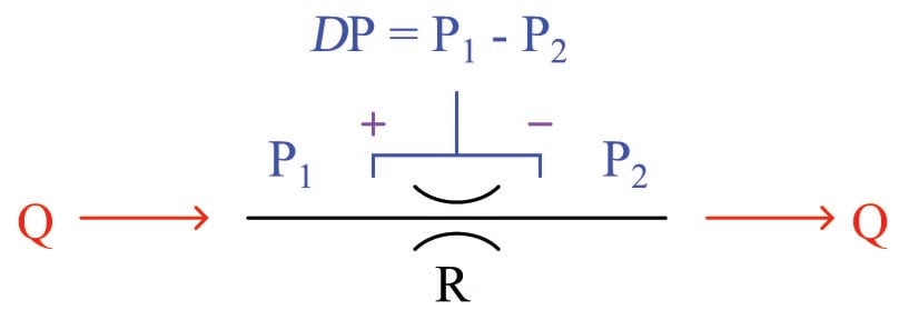
This pressure drop (\(P_1 - P_2\), or \(\Delta P\)) is equivalent to the voltage drop seen across any current-carrying resistor and may be substituted for dissipated energy per unit volume in the previous equation. We may also substitute \(Q \over A\) for velocity \(v\) because we know volumetric flow rate (\(Q\)) is the product of fluid velocity and pipe cross-section area (\(Q = Av\)) for incompressible fluids such as liquids:
\[P_1 - P_2 = {1 \over 2} k \rho \left(Q \over A\right)^2\]
Next, we will solve for a quotient with pressure drop (\(P_1 - P_2\)) in the numerator and flow rate (\(Q\)) in the denominator so the equation bears a resemblance to Ohm’s Law (\(R = {V \over I}\)):
\[P_1 - P_2 = {1 \over 2} k \rho {Q^2 \over A^2}\]
\[{{P_1 - P_2} \over Q^2} = {k \rho \over 2 A^2}\]
\[{\sqrt{P_1 - P_2} \over Q} = \sqrt{k \rho \over 2 A^2}\]
Either side of the last equation represents a sort of “Ohm’s Law” for turbulent liquid restrictions: the left-hand side expressing fluid “resistance” in the state variables of pressure drop and volumetric flow, and the right-hand term expressing fluid “resistance” as a function of fluid density and restriction geometry. We can see how pressure drop (\(P_1 - P_2\)) and volumetric flow rate (\(Q\)) are not linearly related as voltage and current are for resistors, but that nevertheless we still have a quantity that acts like a “resistance” term:
\[R = {\sqrt{P_1 - P_2} \over Q} \hbox{\hskip 100pt} R = \sqrt{k \rho \over 2 A^2}\]
Where,
\(R\) = Fluid “resistance”
\(P_1\) = Upstream fluid pressure
\(P_2\) = Downstream fluid pressure
\(Q\) = Volumetric fluid flow rate
\(k\) = Turbulent energy dissipation factor
\(\rho\) = Mass density of fluid
\(A\) = Cross-sectional area of restriction
The fluid “resistance” of a restriction depends on several variables: the proportion of kinetic energy lost due to turbulence (\(k\)), the density of the fluid (\(\rho\)), and the cross-sectional area of the restriction (\(A\)). In a control valve throttling a liquid flow stream, only the first and last variables are subject to change with stem position, fluid density remaining relatively constant.
[fluid_restrictions]
In a wide-open control valve, especially valves offering a nearly unrestricted path for moving fluid (e.g. ball valves, eccentric disk valves), the value of \(A\) will be at a maximum value essentially equal to the pipe’s area, and \(k\) will be nearly zero. In a fully shut control valve, \(A\) is zero, creating a condition of infinite “resistance” to fluid flow.
It is customary in control valve engineering to express the “restrictiveness” of any valve in terms of how much flow it will pass given a certain pressure drop and fluid specific gravity (\(G_f\)). This measure of valve performance is called flow capacity or flow coefficient, symbolized as \(C_v\). A greater flow capacity value represents a less restrictive (less “resistive”) valve, able to pass greater rates of flow for the same pressure drop. This is analogous to expressing an electrical resistor’s rating in terms of conductance (\(G\)) rather than resistance (\(R\)): how many amperes of current it will pass with 1 volt of potential drop (\(I = GV\) instead of \(I = {V \over R}\)).
If we return to one of our earlier equations expressing pressure drop in terms of flow rate, restriction area, dissipation factor, and density, we will be able to manipulate it into a form expressing flow rate (\(Q\)) in terms of pressure drop and density, collecting \(k\) and \(A\) into a third term which will become flow capacity (\(C_v\)):
\[P_1 - P_2 = {1 \over 2} k \rho {Q^2 \over A^2}\]
First, we must substitute specific gravity (\(G_f\)) for mass density (\(\rho\)) using the following definition of specific gravity:
\[G_f = {\rho \over \rho_{water}}\]
\[\rho_{water} G_f = \rho\]
Substituting and continuing with the algebraic manipulation:
\[P_1 - P_2 = {1 \over 2} k \rho_{water} G_f {Q^2 \over A^2}\]
\[{{P_1 - P_2} \over G_f} = {1 \over 2} k \rho_{water} {Q^2 \over A^2}\]
\[\left({2 A^2 \over k \rho_{water}}\right) \left({{P_1 - P_2} \over G_f}\right) = Q^2\]
\[Q = \sqrt{2 A^2 \over k \rho_{water}} \> \sqrt{{P_1 - P_2} \over G_f}\]
The first square-rooted term in the equation, \(\sqrt{2 A^2 \over k \rho_{water}}\), is the valve capacity or \(C_v\) factor. Substituting \(C_v\) for this term results in the simplest form of valve sizing equation (for incompressible fluids):
\[Q = C_v \sqrt{{P_1 - P_2} \over G_f}\]
In the United States of America, \(C_v\) is defined as the number of gallons per minute of water that will flow through a valve with 1 PSI of pressure drop. A similar valve capacity expression used with metric units rates valves in terms of how many cubic meters per hour of water will flow through a valve with a pressure drop of 1 bar. This latter flow capacity is symbolized as \(K_v\).
For the best results predicting required \(C_v\) values for control valves in any service, it is recommended that you use valve sizing software provided by control valve manufacturers. The formulae shown here do not account for all factors influencing fluid flow rate and pressure drop and therefore yield approximate values only. Modern valve sizing software is easy to use, especially when referenced to specific models of control valve sold by that manufacturer, and is able to account for a diverse multitude of factors affecting proper sizing.
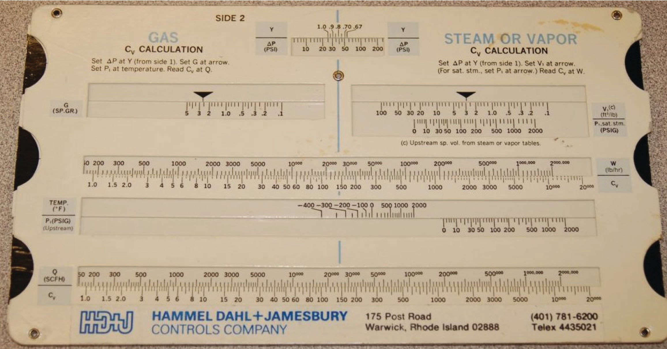
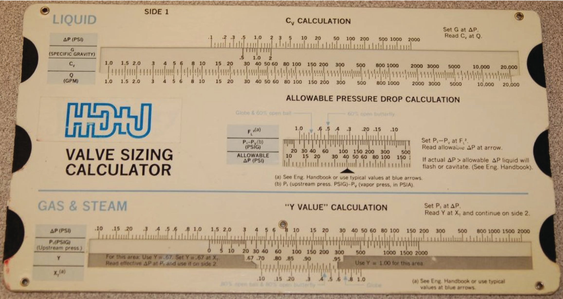
Control valve sizing is complex enough that some valve manufacturers used to give away “slide rule” calculator devices so customers could choose the \(C_v\) values they needed with relative ease. Photographs of a two-sided valve sizing slide rule are shown here for historical reference:
Importance of Proper Valve Sizing
The flow coefficient of a control valve (\(C_v\)) is a numerical value expressing the number of gallons per minute flow of water the valve will pass with a constant pressure drop of 1 PSI from inlet to outlet. This rating is usually given for the valve in its wide-open state. For example, a control valve with a \(C_v\) rating of 45 should flow 45 gallons per minute of water through it with a 1 PSI pressure drop when wide open. The flow coefficient value for this same control valve will be less than 45 when the valve position is anything less than fully open. When the control valve is in the fully shut position, its \(C_v\) value will be zero. Thus, it should be understood that \(C_v\) is truly a variable – not a constant – for any control valve, even though control valves are often specified simply by their maximum flow capacity.
As previously shown, the basic liquid-flow equation relating volumetric flow rate to pressure drop and specific gravity is:
\[Q = C_v \sqrt{{P_1 - P_2} \over G_f}\]
Where,
\(Q\) = Volumetric flow rate of liquid (gallons per minute, GPM)
\(C_v\) = Flow coefficient of valve
\(P_1\) = Upstream pressure of liquid (PSI)
\(P_2\) = Downstream pressure of liquid (PSI)
\(G_f\) = Specific gravity of liquid (ratio of liquid density to standard water density)
A common misconception is that \(C_v\) represents an absolute maximum flow rating for a valve. This is not true, any more than the resistance value of an electrical resistor reflects some maximum current value for that component. It is possible – at least in theory – to shove any rate of flow through any open valve given enough pressure to motivate that flow. \(C_v\), like electrical resistance measured in ohms, merely states the proportion between flow rate and pressure drop. \(C_v\) is simply the maximum flow rate of water through a control valve given a 1 PSI pressure difference from upstream to downstream.
It should be obvious that any control valve must be sized large enough (i.e. possess sufficient maximum \(C_v\) capacity) to flow the greatest expected flow rate in any given process installation. A valve that is too small for an application will not be able to pass enough process fluid through it given the fluid pressure available.
Given this fact, it may seem safe to choose a valve sized much larger than what is needed, just to avoid the possibility of not having enough flow capacity. For instance, consider this control valve sizing problem, where a characterized ball valve controls the flow rate of water out of a surge tank to maintain a constant water level 25 feet higher than the height of the valve:
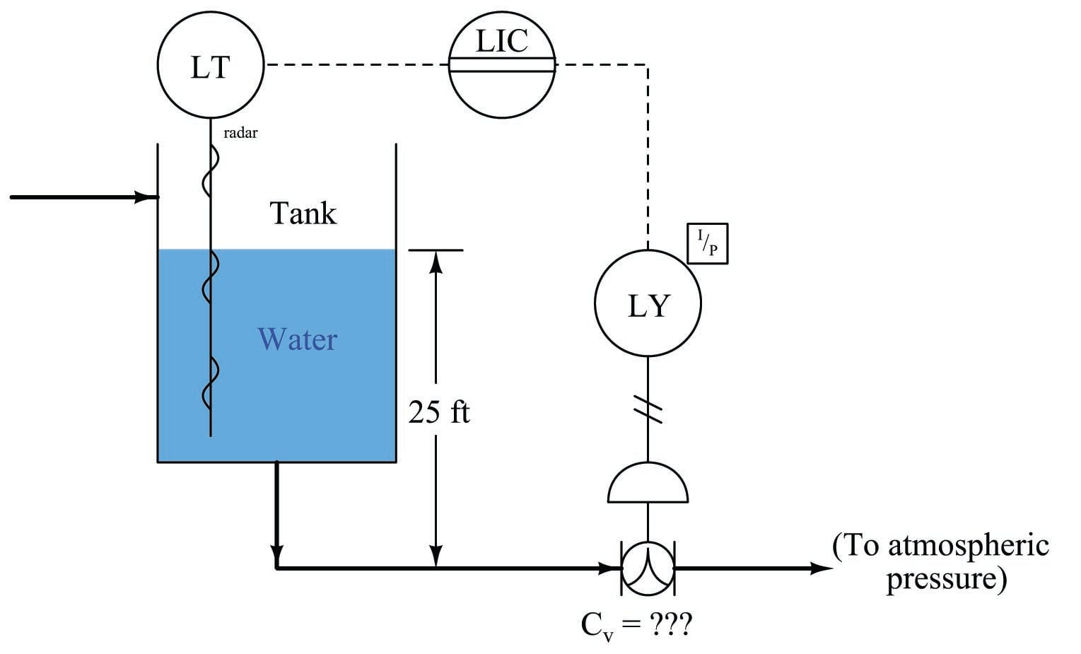
Suppose the process engineer designing this system specifies a maximum flow rate for this valve of 470 GPM. What should the maximum \(C_v\) rating be for this valve? To begin, we must know the expected pressure drop across the valve. The 25-foot water column height upstream provides us with the means to calculate \(P_1\) by using the formula for calculating hydrostatic pressure (the pressure generated by a vertical column of liquid under the influence of gravity):
\[P = \gamma h\]
\[P_1 = (\hbox{62.4 lb/ft}^3)(\hbox{25 feet})\]
\[P_1 = 1560 \hbox{ PSF} = 10.8 \hbox{ PSI}\]
There is no need to calculate \(P_2\), since the P&ID reveals the downstream side of the valve to be vented to atmosphere, and thus is guaranteed to be 0 PSI gauge pressure. This gives us a pressure drop of 10.8 PSI across the control valve, with an expected maximum flow rate of 470 GPM. Manipulating our flow capacity equation to solve for \(C_v\):
\[Q = C_v \sqrt{{P_1 - P_2} \over G_f}\]
\[C_v = {Q \over \sqrt{{P_1 - P_2} \over G_f}}\]
\[C_v = {470 \hbox{ GPM} \over \sqrt{{10.8 \hbox{ PSI}}\over 1}}\]
\[C_v = 143\]
This tells us we need a control valve with a \(C_v\) value of at least 143 to meet the specified (maximum) flow rate. A valve with insufficient \(C_v\) would not be able to flow the required 470 gallons per minute of water with only 10.8 PSI of pressure drop. As mentioned previously, these calculations yield approximate results only. An analysis using computer-based valve sizing software may require an even larger control valve for this application.
Does this mean we should over-size the valve, just to ensure we don’t install one that is too small? For the sake of argument, would there be any problem with installing a control valve with a \(C_v\) value of 300? The general answer to these questions is that over-sized valves may create other problems. Not only is there the possibility of allowing too much flow under wide-open conditions (consider whatever process vessels and equipment lie downstream of the oversized valve), but also that the process will be difficult to control under low-flow conditions.
In order to understand how an over-sized control valve leads to unstable control, an exaggerated example is helpful to consider: imagine installing a fire hydrant valve on your kitchen sink faucet. Certainly, a wide-open hydrant valve would allow sufficient water flow into your kitchen sink. However, due to the gross mismatch between a fire hydrant valve’s flow capacity versus that of relatively skinny tubing providing water to the sink faucet, most of this valve’s usable range of throttling will be limited to the first percent of stem travel. After the valve is opened just a few percent from fully shut, restrictions in the piping of your house’s water system will have limited the flow rate to its maximum, thus rendering the rest of the valve’s stem travel capacity utterly useless. It would be challenging indeed to try filling a drinking cup with water from this hydrant valve: just a little bit too much stem motion and the cup would be subjected to a full-flow stream of water!
An over-sized valve is, therefore, an overly-sensitive valve from the perspective of the control system driving it. With the upper end of the valve’s travel being useless for control (having little or no effect), all the throttling action must take place within the first few percent of stem motion. This makes precise control of the flow rate more challenging than it should be. Typical valve problems such as stem friction, hysteresis, and calibration error, therefore, become amplified when the valve is over-sized because any amount of imprecision in stem positioning becomes a greater percentage of the valve’s useful travel range than if the valve were properly sized and able to use its full range of motion.
Control valve over-sizing is a common problem in the industry, often created by future planning for expanded process flow. “If we buy a large valve now,” so the reasoning goes, “we won’t have to replace a smaller valve with a large valve when the time comes to increase our production rate.” In the interim period when that larger valve must serve to control a meager flow rate, however, operational problems caused by poor control quality may end up costing the business more than the cost of an additional valve. The key here, as in so many other applications in business, is to carefully consider costs over the life-span of the device, not just the initial (capital) expense.
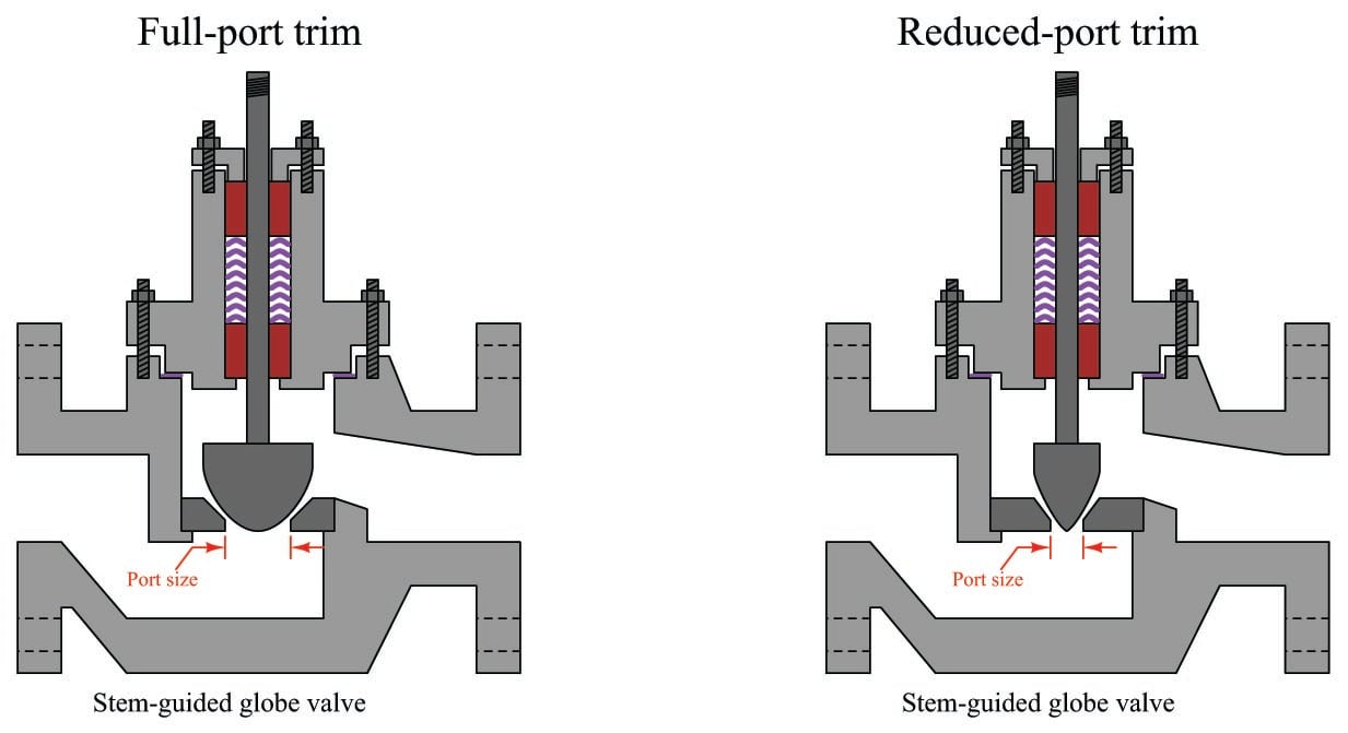
A practical solution to the problem of valve over-sizing – especially when larger flow rates will be required of the valve in the future – is to initially order the control valve with a body size suitable for the largest flow capacity it will need in the future, but equipped internally with reduced-port (or restricted-capacity) trim. This means trim having smaller holes (“ports”) through which the fluid must flow. Such a “reduced” trim is under-sized for the valve body, making the control valve’s \(C_v\) rating significantly less than it would be with normal-sized trim installed. The benefit of installing reduced-port trim in a control valve is that the flow capacity of the valve may be upgraded simply by removing the reduced trim components and replacing them with full-port (full-sized) trim. Upgrading a control valve’s trim to full-port size is significantly less expensive than replacing the entire control valve with a larger one.
Reduced-port trim for a stem-guided or port-guided globe valve takes the form of a new (smaller) plug and seat assembly. The seat is specially designed to match the plug for tight shutoff and good throttling behavior while having the necessary external dimensions to fit the larger valve body casting:
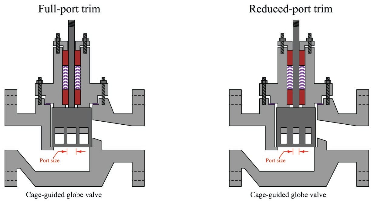
Reduced-port trim for a cage-guided globe valve often consists of nothing more than a new cage, having smaller ports in the cage than standard. Thus, reduced-port trim for a cage-guided globe valve may utilize the exact same plug and seat as the full-port trim for the same cage-guided globe valve:
Gas Valve Sizing
Sizing a control valve for gas or vapor service is more complicated than for liquid service, due to the compressibility of gases and vapors. As a gas or vapor compresses with changes in pressure, its density changes correspondingly. In previous mathematical analyses of fluid flow restriction, one of our assumptions was that fluid density (\(\rho\)) remained constant. This assumption may hold true for some flowing gas conditions as well, provided minimal pressure changes within the path of flow. However, for most gas control valve applications where the very purpose of the valve is to introduce substantial pressure changes, the assumption of constant gas density is unrealistic.
Shown here is one of the simpler gas valve sizing equations you will encounter:
\[Q = 963 \> C_v \sqrt{{\Delta P (P_1 + P_2)} \over {G_g T}}\]
Where,
\(Q\) = Gas flow rate, in units of Standard Cubic Feet per Hour (SCFH)
\(C_v\) = Valve capacity coefficient
\(\Delta P\) = Pressure dropped across the valve, pounds per square inch differential (PSID)
\(P_1\) = Upstream valve pressure, pounds per square inch absolute (PSIA)
\(P_2\) = Downstream valve pressure, pounds per square inch absolute (PSIA)
\(G_g\) = Specific gravity of gas (ratio of gas density to standard air density)
\(T\) = Absolute temperature of the gas in degrees Rankine (\(^{o}\)R), equal to degrees Fahrenheit plus 459.67
This equation holds true only for “subcritical” flow, where the moving gas stream velocity never approaches the speed of sound. Other equations exist for calculating flow rates of gas through control valves in the presence of sonic flow regimes. Note the inclusion of absolute pressures in this equation, and not just differential pressure (\(\Delta P\), or \(P_1 - P_2\)). This is intended to correct for effects related to compression of the gas under pressure.
Valve sizing is complicated enough, both for liquid and gas service, that the use of valve sizing computer software is strongly recommended as opposed to hand-calculations. The number of important parameters, nonlinear factors, and alternative equations relevant to control valve sizing are numerous enough to bewilder most technicians (and more than a few engineers). Valve sizing software will also predict noise levels generated by the valve, and in many cases specify actual valve trim styles offered by the manufacturer for mitigating problems such as noise.
Relative Flow Capacity
The flow capacity of a valve (\(C_v\)) is a quantitative rating of its ability to pass a fluid flow for a set of given pressure and fluid density conditions, defined as the flow rate of water in gallons per minute through the valve given a constant pressure drop of 1 PSID. \(C_v\) may be predicted, or empirically measured, for any type of control valve given the proper information.
Not all control valve types exhibit the same \(C_v\) coefficients, however, for the same pipe size. A 4-inch butterfly valve, for example, has a much greater full-open \(C_v\) rating than a 4-inch globe valve, due to the much more direct path it offers to a moving fluid. A simple comparison of these two valve types clearly shows why this is true (note the “constriction” points labeled with arrows):
A globe valve is simply more effective at generating fluid turbulence – and therefore dissipating fluid kinetic energy – than a butterfly valve of the same pipe size, because the globe valve design forces the fluid to change direction more often and in different ways.
One way to help quantify a particular valve design’s ability to throttle fluid flow is to express this ability as a ratio of flow coefficient (\(C_v\)) versus a cross-sectional pipe area. The basic principle here is that we should expect the \(C_v\) of any particular valve design to be proportional to pipe area (e.g. a ball valve with twice the pipe area should have twice the flow capacity, all other factors being equal), and therefore a ratio of these two quantities should be fairly constant for any valve design. Since we know the area of a pipe is proportional to the square of either radius or diameter (\(A = {\pi d^2 \over 4}\) or \(A = \pi r^2\)), we may simplify this ratio by omitting all constants such as \(\pi\) and simply relating \(C_v\) factor to the square of pipe diameter (\(d^2\)). This ratio is called the relative flow capacity, or \(C_d\):
\[C_d = {C_v \over d^2}\]
Several approximate valve capacity factors (\(C_d\)) for different control valve types are shown here, assuming full-area (not reduced-port) trim, a wide-open position, and diameter measured in inches:
| Valve design type | \(C_d\) |
|---|---|
| Single-port globe valve, ported plug | 9.5 |
| Single-port globe valve, contoured plug | 11 |
| Single-port globe valve, characterized cage | 15 |
| Double-port globe valve, ported plug | 12.5 |
| Double-port globe valve, contoured plug | 13 |
| Rotary ball valve, segmented | 25 |
| Rotary ball valve, standard port (diameter approx 0.8d) | 30 |
| Rotary butterfly valve, 60°, no offset seat | 17.5 |
| Rotary butterfly valve, 90°, offset seat | 29 |
| Rotary butterfly valve, 90°, no offset seat | 40 |
To calculate the approximate \(C_v\) for any valve, all we need to do is square that valve’s pipe diameter (in inches) and multiply by the valve type’s relative flow capacity (\(C_d\)):
\[C_v \approx d^2 C_d\]
Based on the figures in this table, for example, we may predict that a segmented ball valve with a pipe size of 3 inches will have a flow capacity (\(C_v\)) of approximately 225, or that a single-port cage-guided globe valve with an 8-inch pipe size will have a \(C_v\) of approximately 960.
As you can see from a comparison of \(C_d\) values, a no-offset butterfly valve has nearly 4 times the flow capacity of a single-ported contoured-plug globe valve of the same pipe size (\(C_d\) = 40 versus \(C_d\) = 11). This makes butterfly valves advantageous in applications where large flow capacities must be achieved at minimal costs, such as in air handling (HVAC) systems for commercial buildings and combustion air controls for large industrial burners.
At first glance this may seem to make larger \(C_d\) valve types the superior choice for control valve applications, yielding the greatest \(C_v\) values for the smallest pipe sizes. However, there are other factors to consider such as ease of maintenance, noise and cavitation abatement, characterization, and valve seat leakage. For these reasons, some of the lowest-\(C_d\) valve types (e.g. globe valves) remain popular choices for industrial control applications even though they require larger pipe sizes to achieve the same amount of flow compared to other valve types (e.g. ball valves).
Interested in more information about fluid control and valves?
Check out our fluid calculators:
Related Textbook Pages:
Related Technical Articles:
- Info Byte: Definition of Pressure and Flow in Fluid Systems
- Barg vs Bara: Understanding Absolute and Gauge Pressure
- Common Control Valve Issues and Troubleshooting
