Tutorial: Using SMC E-Actuators with a PLC

Electric actuators are considered superior to pneumatic systems in many ways. Although they may lack some of the brute power/size ratio characteristics of fluid power, electric motion axes provide excellent speed, position, and acceleration profiles, as well as feedback that allows incredibly precise and controllable motion.

Many electric axes require complex setup through a servo motor drive configuration software, often with a USB or fieldbus connection. To simplify the process, SMC offers a somewhat unique offering: the e-Actuator catalog, which uses only PNP/NPN input signals to drive motion to an exact position, much like a pneumatic cylinder with a solenoid valve. Even better, the exact stopping positions can be adjusted easily without requiring any new position feedback sensors.

Working with these actuators as a stand-alone system has been discussed in previous articles, so in this example, we will connect these actuators to a PLC and implement a few simple controls.

Connecting the e-Actuator to the PLC

The first consideration for working with the e-Actuator series is the lack of a common ground on the M12 cable that receives the signal inputs. This was also addressed in a previous article, but to solve the problem, we’ll simply need to span a common neutral (- VDC) wire between the e-Actuator system and the PLC system, assuming they are not both powered by a single DC supply.

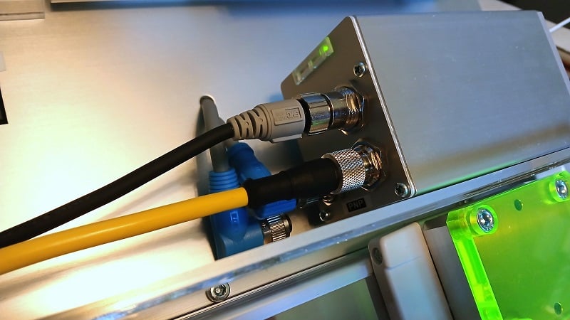
Figure 1. The 8-pin M12 connector for the digital input signals.

The e-Actuator uses an 8-pin M12 connector, so be sure to properly interpret both the pin layout for the actuator (Fig. 1, left side) and match it with the proper wire color layout (Fig. 1, right side). There are industry standards, but there are also variations of the standard.

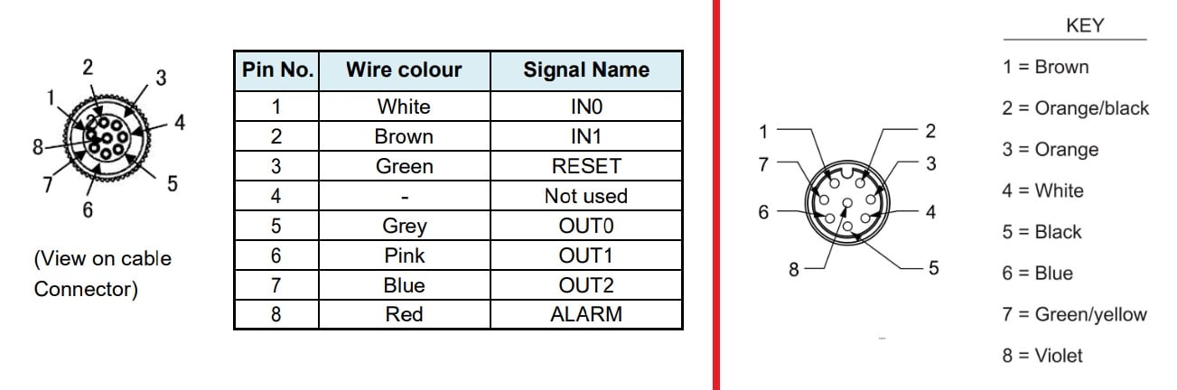
Figure 2. The standard wire colors and the function of the pins listed in the SMC e-Actuator manual (left) and an example of a slightly different wire color pinout from a major manufacturer (right) (source).

For this example, we need to access signals IN0 and IN1, at a minimum. Because my cable is shown on the right, this means that I need to connect the brown wire (pin 1) and the orange/black wire (pin 2) to the PLC output module.

In summary:

• (- V) of e-Actuator system <--> (- V) of PLC system
• Pin 1, IN0 of the e-Actuator <--> Brown wire of M12 cable <--> PLC Output 0
• Pin 2, IN1 of the e-Actuator <--> Or/Blk wire of M12 cable <--> PLC Output 1

Addressing Feedback Signals

Another helpful feature of this e-Actuator system is the adjustable limits with feedback signals that do not require any manual adjustment of sensors. According to the wiring diagram in Fig. 1, we can connect OUT0, OUT1, and OUT2 over to the input terminals of the PLC.

When the actuator reaches the near end of its configured stroke, OUT0 will energize. Likewise, when the actuator reaches the far end, OUT1 energizes. When it reaches the center point, OUT2 will energize.

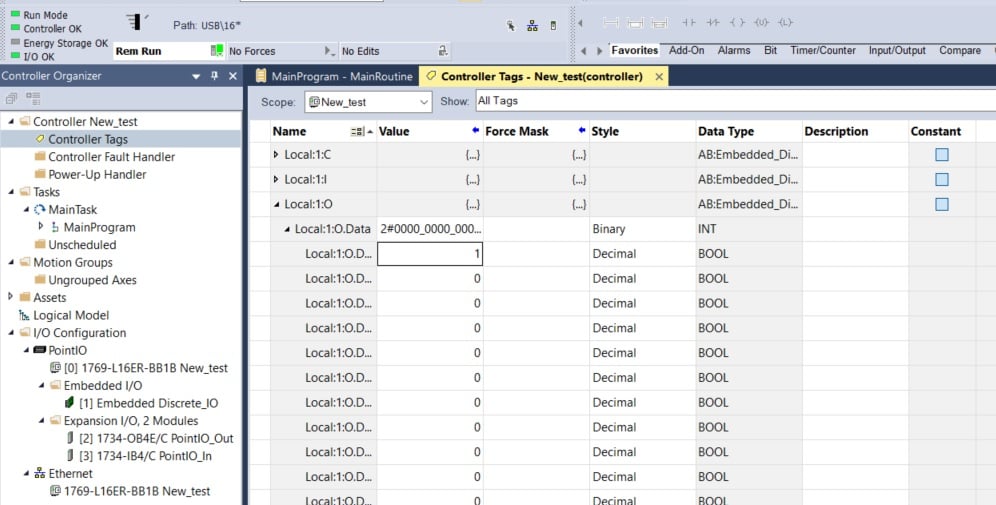
Figure 3. The tag listing that sends output signals into the e-Actuator’s IN0 and IN1 inputs.

Testing the Tags

This tutorial can be applied to virtually any PLC with digital discrete outputs, but my scenario uses an Allen-Bradley L16 PLC with embedded digital I and O.

Once the wires were connected and both the PLC system and the actuator system were powered on, it is time to test the function of the system.

Navigate to the global tags and find the output module, which for this embedded system is Local:1:O.Data. Toggling bit 0 will move the actuator to the near end of its stroke. Toggling bit 1 will move the actuator to the far end. Activating both bits should move it to the center of the stroke. This all assumes you have completed my first tutorial for configuring the e-Actuator and placing it into ‘closed center’ operating mode.

A Basic Program

This program will use three momentary pushbuttons, one for each position.

The logic of the program will cause one or both of the outputs to energize when the buttons are pressed. Make sure not to use the same output in two different rungs.

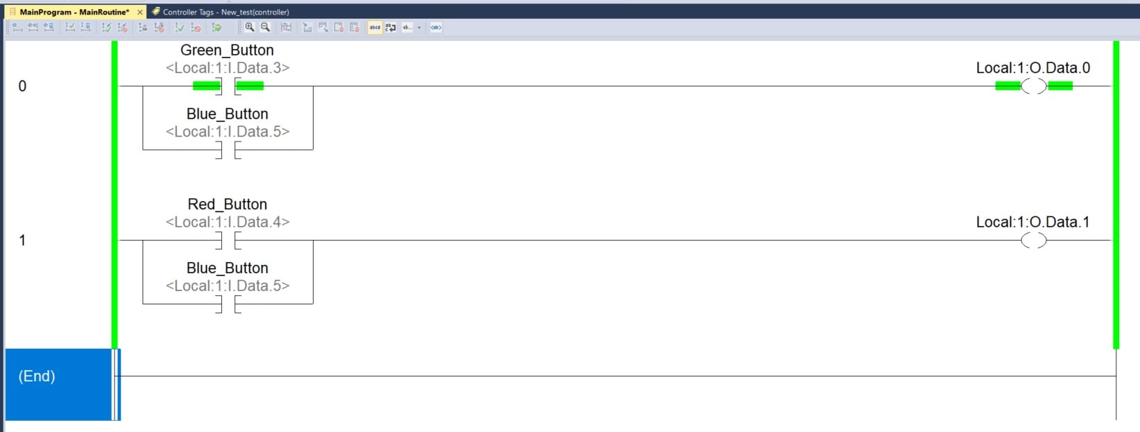
Figure 4. A 2-rung program to operate one or both digital outputs.

Using the Feedback Signals

This simple program didn’t incorporate the inputs from the e-Actuators, but they can be used to gain valuable information. Particularly with timers:

1. If a command is given to move from the near end to the far end of the actuator, the configuration of the actuator should determine exactly how long this action should take. A timer with a preset of this time could be used as a warning flag that the actuator may be overloaded or jammed. In other words, something is causing a major problem right now.
2. If the elapsed time between motions is recorded each time the command is given, this record can be examined for potential wear or needed maintenance for the system. In other words, something is causing a gradual problem over a period of time.

Electric Motion

As with any automation system, the costs of the system must be weighed against the return on the investment. Electric actuators are more costly, and, typically, are more complex to operate. This product series provides an interesting example that removes one of those barriers, making the concept of electric actuation more appealing, even for simple projects.