Finding and Calibrating Linear Regression in LabVIEW

The real world is made of analog signals, such as temperature, pressure, fluid level, flow rate, luminosity, or any number of other natural phenomena. These analog signals are translated to a voltage or current that can be interpreted by the data acquisition system and the computer into something usable by human control operators.

Take, for example, simple temperature measurement with a thermocouple. As the process temperature changes, the Seebeck effect generates a different voltage across the thermocouple terminals. If the thermocouple is appropriate for the process temperatures, the voltage will vary linearly with temperature. 

 

Figure 1. A thermocouple in an industrial heating system.

 

Engineers and technicians can use a simple linear equation of the form y = mx + b to determine the temperature of the thermocouple (y) based on the voltage (x). They can determine the slope (m) and the y-intercept (b) by creating a best-fit line from raw data.

 

Collecting Raw Data

To find the equation of the best-fit line, the engineer or technician must first collect data. To collect this data, the instrumentation system should be connected to measure the voltage or current from the sensor directly. A secondary, trusted sensor is placed in the same environment, such that it can be read visually at the same time as the voltage from the first sensor.

When calibrating a thermocouple, the engineers and technicians can place a glass thermometer in the same environment and read its temperature. This temperature corresponds to the voltage read from the sensor. 

Repeat this process under different environments. A thermocouple can be placed in a water bath with a glass thermometer and heated on a hot plate, as an example. The technician can take temperature and voltage measurements and build a calibration table.

Ideally, data points should be taken at random. This minimizes the effects of sampling limitations and biases that occur as an experiment is conducted in a specific order. However, in some cases, it may be more cost-effective to take the measurements in a set order. It can be easier to take temperature measurements during a heating cycle than randomly pick temperatures, wait for the temperature to stabilize, then take a voltage measurement at each of these points.

One way to minimize these effects is to take many data points, repeat the experiment frequently, and update the calibration as needed. Also, experiments can be conducted in reverse to check for hysteresis. Maybe the temperature measurements are taken as the water bath heats up, but then take them again as it cools off and see how the measurements compare.

 

Finding a Best-fit Line

When using a spreadsheet program plot, all of the voltages and measurements on an x and y planes, respectively. Then, in the spreadsheet program, there will be an option to create a best-fit line. The best-fit line equation can be displayed, and it should show some equation of the form y = mx + b.  Mathematically, the technician could predict the temperature by reading the voltage and entering it for x in this equation.

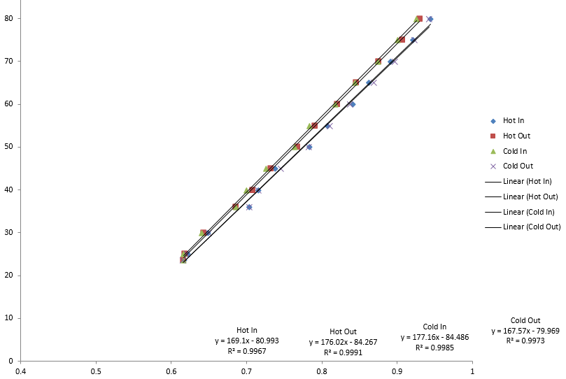
Figure 2. This graph shows the voltage versus temperature for four thermocouples. 

 

In figure 2, notice how all four thermocouples have an associated equation that meets the form y = mx + b. Also, notice how all four thermocouples are very similar but not identical, which is expected from four similar thermocouples.

 

How to Calculate R^2 Value

Some software packages offer neat, but often abused, options. For example, there is often an option to display the “R^2” value. Skipping the long mathematical explanation, the R^2 value can be thought of as a way to measure the linearity of the data or how closely the best-fit line approximates the value of the measurement. A value of 1 would indicate a perfect fit, and a value of 0 is no fit at all. 

Real data is often sloppy. While the graph above has nice R^2 values of nearly 1, sometimes that isn’t the case. Maybe the R^2 values are closer to 0.7 or a similar number. Unfortunately, many technicians and engineers treat an R^2 value equal to 1 as a gold standard to which all data should match. This is not the case. Hopefully, adding more data points will legitimately increase the R^2 value.

Where engineers and technicians can get into trouble is by changing the equation order. If a line does not fit well, it may be tempting to try to model it with a parabola, cubic, or another polynomial instead. If they do this, they will get an R^2 value of 1, as they will have found a polynomial that snakes through every data point. This is a poor practice and does not represent reality. Instead, they should know enough about the behavior of the sensor (linear, exponential, quadratic, etc.) and use only the proper order. 

 

Calibration in LabVIEW

At this point, there is a graph and an equation that represents how the sensor voltage (or current) will change with a changing environment. LabVIEW can convert the raw sensor data into human-readable data on the graphical user interface (GUI).

In the case of a linear sensor, the programmer can simply feed the raw data into a multiplication terminal, where it will be multiplied by the slope (m) from the best-fit line. This number can be wired to an addition terminal. The other terminal can be wired to a constant with the b value.

 

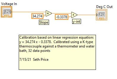
Figure 3. In this case, the equation is y = 34.274 x - 0.3378. In a full program, the “voltage in” may come directly from a data processing sub-VI.

 

From here, the programmer should create a sub-VI (virtual instrument) that encompasses the math steps. The calibration may be used in multiple parts of the program. As a sub-VI, new calibration data can be entered into the sub-VI alone, and it will perform the proper calculations throughout the VI. If a sub-VI is not used, each instance requires an update, which is time-consuming and often the source of errors.

Finally, the sub-VI should be documented. At the very minimum, include the units, the calibration method, and the name and date of the person who performed the calibration. Documentation can also include serial numbers, part numbers, and other such relevant information.

Linear regression is a powerful tool in instrumentation. Combined with LabVIEW, technicians and engineers can create a calibrated instrumentation system quickly. The engineer should be warned, however, not to abuse the capabilities of their spreadsheet software package.